Advanced Setups

If you need to enhance your model with additional data or details—whether for a better simulation accuracy or improved visual context—or if you're working on larger regions, scenarify’s advanced setup options are the way to go for creating a new model from scratch.

Advanced setup options are especially useful for:

• integrating more complex datasets, such as tiled raster data or collections of rasters with varying resolutions, or
• handling data not available through land use, such as custom building shape files, soil data, or culverts.

Recommended Setup Order

For the key model data and setup steps, it is important to follow the recommended order outlined in the numbered sections below. However, when adding supplementary details like roofs or soil data, the setup sequence becomes more flexible.

Example Setup

For some of the figures and examples, we will continue using the data from the Liesing district of Vienna, as introduced in the Fast Setups section.

1. Create a New Project

In the Project Menu, select New Blank to start a new project from scratch. The View will be initialized with the Setup: Files visual preset, which highlights the file boundaries of each geo-referenced dataset you add to the model.

2. Project Coordinate System

Setup Location: Simulation Settings Panel > Coordinate System

Begin your advanced setup by specifying a coordinate system for your project. Any imported data, regardless of its initial coordinate system, will automatically be transformed into the project coordinate system, ensuring all data layers fit together accurately.

You can define the project coordinate system in two ways:

• Automatic Parsing: Enable the Auto Select Coordinate System checkbox to automatically retrieve the coordinate system from a geo-referenced data file of your choice.
• Manual Entry: Disable the Auto Select Coordinate System checkbox to enter the coordinate system manually. Supported formats include PROJ4, Well-Known Text (WKT), and authority codes like "EPSG:27700" or "WGS84".

Additionally, a translation vector can either be computed automatically from the data file or entered manually. The automatically computed translation vector shifts the coordinates closer to the origin (0,0), ensuring optimal numerical precision.

When retrieved automatically, the coordinate system definition and translation vector values are displayed in their respective fields:

Hint: It is recommended to automatically extract both the coordinate system and translation vector from your terrain raster file, whether you're working with a single file or a tiled raster dataset.

3. Terrain

Setup Location: Simulation Settings Panel > Terrain

Main Raster Source

Specify the main terrain raster source for simulation. The drop-down menu provides several options for defining the main raster:

• Raster Cascade: Consists of one or more layers, with each layer containing an individual raster file. Layers can have different extents, resolutions, and data formats. Initially, the raster cascade contains one empty layer, labeled Element 1. Additional layers can be added using the Add Element button. By default, each layer inherits the settings shown under Default Settings. However, you can override any of these settings for any individual layer by adding settings to a layer:
  
  Click the button to open a drop-down menu for the desired layer. From there, select the settings you want to override, then click Apply. The chosen settings will be displayed for the layer, allowing you to adjust them as needed for that layer:
  
  To remove specific settings of a layer, de-select them in the drop-down menu and click Apply.
  The raster cascade algorithm fills each cell of the simulation domain by checking the layers in a top-down sequence. As soon as a valid value is found for a cell, it moves to the next cell, ensuring that the first available value is used. Therefore, the order of raster cascade layers is important.

• Raster Tiles: Uses one or more directories containing structured, regular sets of raster tiles, with tiles in the same directory sharing the same coordinate system. Directories can be added using the Add Directory Path button:
  When generating the heightfield from raster tiles, scenarify prioritizes the directories as they appear in the sequence (top to bottom). Within each directory, tiles are processed alphabetically. If Reorder Tiles According to Resolution is enabled, higher-resolution tiles are favored over lower-resolution ones, while preserving the original order for tiles with the same resolution.

Similar to a raster cascade, the system traverses the simulation grid cell by cell. For each cell, it checks the tiles in order and uses the first available value it finds. Once a value is assigned to a cell, the algorithm stops searching further layers.

• SMS Mesh (.2dm): Uses a irregular mesh file to derive the terrain raster. scenarify requires a user-specified coordinate system for proper processing.

• MIKE (.dfs2, .dfsu): Extracts terrain data from a file produced by the MIKE modeling software. Currently only limited support, error-free reading of files from all MIKE versions cannot be guaranteed.

Secondary Raster Source

This option allows you to specify an additional terrain raster source, which will be used in areas where the main terrain raster is not available. The secondary raster can be sourced from either a raster cascade or raster tiles, operating similarly to the Main Raster Source group.

Automatic Raster

The automatic raster is the default terrain raster when using a pre-built base model. It can be used to fill gaps or extend the main raster coverage. However, the main raster always takes precedence over the automatic raster.

4. Domains

Setup Location: Action Tool Selector > Domain Setup

In scenarify, models use three nested domains, each with a different level of detail, as described in the Fast Setups section. When setting up domains in your model, the following steps are recommended:

1. Assign the Maximum Simulation Domain: Set the maximum simulation domain to match the file bounds of the main raster file or the raster tiles. If necessary, reduce the resolution by increasing the cell size to improve performance. For more details, refer to the documentation on the Maximum Simulation Domain action.

2. Set the Simulation Domain: Place the simulation domain within the bounds of the maximum simulation domain with a mouse click. For advanced configurations (e.g., polygonal domains), refer to the documentation on the Simulation Domain action.

3. Configure the Decorative Domain: Load surrounding terrain data at a lower resolution by configuring the secondary raster source. If this terrain data is only needed for visualization purposes, make sure to disable it for simulation in the Loading Domains (Optimizations) section of Terrain settings. For more details, refer to the documentation on the Decorative Domain action.

5. Land Use

Setup Location: Simulation Settings Panel > Landuse

In scenarify land use data is utilized to derive key model parameters such as surface roughness coefficients, while also enhancing the visual context within the 3D scene.

Land Use Shape Files

The land use shape file should include an attribute specifying the land use type per polygon (e.g., forest, parking lot, building). Users must indicate this attribute by selecting it from a drop-down menu, as shown in the Fast Setups section.

Hint: When working with larger domains, consider displaying land use data only within the simulation domain to improve performance.

Mapping Land Use Types to Visual and Model Parameters

Land use polygons provide terrain coverage, and depending on their type (e.g., forest, construction site, parking lot), specific localized model parameters and visual properties are assigned. These assignments are based on user-configured mappings, with each land use type corresponding to a specific combination of parameters. Different modeling components use their own mappings to define the relevant model parameters:

Component	Mapping Setup Location	Mapped Parameters
Surface roughness	Simulation Settings Panel > Surface: Roughness	Manning's roughness (Roughness)
Interception	Simulation Settings Panel > Surface: Interception (Zones)	Interception storage capacity (Cap) and interception rate (Rate)
Infiltration	Simulation Settings Panel > Soil: Infiltration Zones	Saturated hydraulic conductivity (Sat Con), suction head along the wetting front (Suct Head), and difference porosity (Diff Por)
Visual context	Simulation Settings Panel > Landuse	Terrain color, opacity, and texture (no influence on simulation)

Assuming the project is set up as in the Fast Setups section, we will use the surface roughness component as an example to demonstrate you how to work with land use type mappings. In the Simulation Settings Panel under Surface: Roughness, the group Landuse Roughness from displays a predefined mapping from land use types to roughness values in Strickler units:

The "Landuse" column contains land use types from the vocabulary of the Austrian cadastral system BEV. The "Roughness" column lists the corresponding roughness values pre-calibrated by the scenarify team. If needed, you can modify individual roughness values to better suit your project. Other predefined land use vocabularies are available in scenarify from the drop-down menu under Landuse Roughness from, including ALKIS (Germany) and OSM (global). Utilizing one of these vocabularies accelerates the setup process, as appropriate model parameters for each land use type are already predefined, eliminating the need to manually assign them.

Hint: For a land use type mapping to function correctly, the mapped land use types must correspond to those present in the actual land use shape file. Therefore, not every vocabulary is suitable for every land use shape file.

Custom mappings can also be used, but they require manual configuration of model parameters. In the drop-down menu under Landuse Roughness from, switch to "Custom Landuse". The custom mapping is initially empty. New elements can be added to the mapping using the Add Element button:

After adding a new element, select a land use type from the drop-down menu in the "Landuse" column. Initially, the land use type choices will be empty. To populate them, toggle the Disable Update of Landuse Choices checkbox off and then on again. This allows the system to read the land use data and identify the available types. This step only needs to be performed once:

After selecting a land use type, input the desired value for that type. You can also import a value from one of the predefined vocabularies mentioned earlier. When entering a roughness value, mind the checkbox above indicating whether the value should be interpreted in Manning or Strickler units:

Keep adding elements until all the desired land use types are covered.

Hint: If a land use type exists in the shape file but is not included in the mapping, the corresponding terrain areas will be assigned default parameter values for the respective model component, as configured in the settings. The same applies when a land use type is disabled in the mapping by toggling the "Use" checkbox off.

For other components, including infiltration, interception, or visual context, land use type mappings are set up in a similar manner. The predefined vocabularies (BEV, ALKIS, and OSM) are also available for these components.

Land Use Synonyms

Different shape files often contain land use types that are named slightly differently but are semantically similar or identical. For example, "parking", "parking lot", and "Parking lot" likely refer to the same land use type but are technically different names. A naïve approach would require adding all such variants to the mapping to ensure coverage. To avoid this redundancy, scenarify supports synonyms for land use types included into the predefined BEV, ALKIS, and OSM vocabularies. Thanks to the synonyms support, "Freizeitfläche" and "Freizeitflächen" will be treated as the same type, sharing the same model parameters and visual appearance.

Land use synonyms for the predefined vocabularies are managed in the Landuse category of the Simulation Settings Panel, under OSM Synonyms, ALKIS Synonyms, or BEV Synonyms, respectively. Users can add new synonyms for the predefined vocabularies if they come across any:

6. Building Footprints

Setup Location: Simulation Settings Panel > Buildings: Footprints

Buildings play a crucial role in river flood and stormwater simulations. They serve as physical barriers to water flow, intercept rainfall, and enhance geospatial visualization, thereby offering important visual context.

Defining Building Source

There are three options for building footprints, selectable under Buildings Source:

• Extract from Landuse: The user should identify which land use types correspond to buildings. Building footprints will then be automatically generated from the land use polygons associated with those specified types:
  

• Buildings Shape File: The user can upload a shape file containing building footprint polygons. Additionally, shape file attributes can be provided to specify ground and roof levels, which are used for generating better 3D building models, as well as building types:
  

• Automatic: The automatic buildings are default when using a pre-built base model.

Visual Context

Setup Location: Visualization Settings Panel > Setup Visual Context

These setup elements do not affect the simulation but enhance user orientation within the 3D model space and contribute to a more visually engaging scene, resulting in improved screenshots, videos, or interactive presentations.

Open Street Maps

The fundamentals of setting up OSM shape files are explained in the Fast Setups section. Additionally, under Open Street Maps (OSM), users can further customize the appearance and visual prominence of elements like roads, railways, or geographic labels:

Vegetation

The Fast Setups section outlines how to generate vegetation based on land use data. The Setup Visual Context: Vegetation category offers more detailed control over the distribution of vegetation types and sizes. Additionally, tree locations can be filtered from the OSM points dataset or imported directly from a cadastral shape file:

It is also possible to specify land use types for vineyards generation.

Administrative Borders

Administrative borders can be loaded from a shape file and displayed directly or selectively, based on an attribute filter:

3D Building Models

Setup Location: Simulation Settings Panel > Buildings: 3D Models

The Fast Setups section explains how to import enhanced 3D building models in CityGML format. These improved models offer more detailed building footprints, resulting in more accurate simulation outcomes. In addition to CityGML, scenarify also supports loading highly detailed, textured 3D models of individual buildings in OBJ format:

Advanced options involve placing the building models manually with interactive handles.

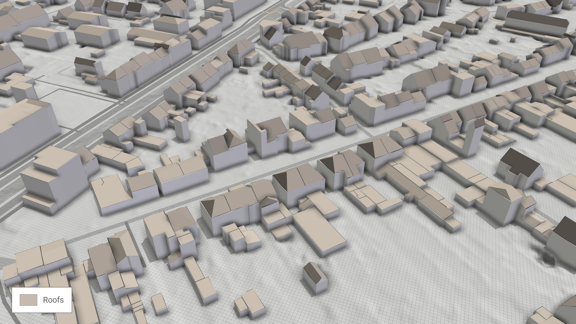
Roofs

Setup Location: Simulation Settings Panel > Buildings: Roofs

To understand how roof water is treated in scenarify, refer to the roof model description. When specifying polygons for roof water computations, the following options are available:

• Building Polygons:
  This is the simplest option. The roof polygons are taken directly from the building footprint polygons. However, in this mode, roof water cannot be directed to specific sewer nodes:
  

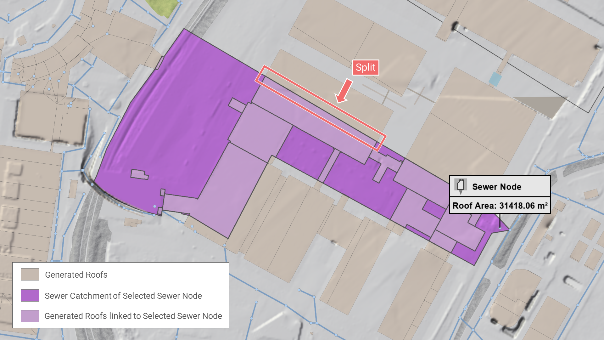
• Building Polygons in Sewer Catchments:
  In this mode, roof polygons are also derived from the building footprint polygons. Roofs are linked to the corresponding sewer node based on the sewer catchment that intersects the roof polygon. If a building overlaps multiple sewer catchments, the roof polygons are automatically split accordingly:
  

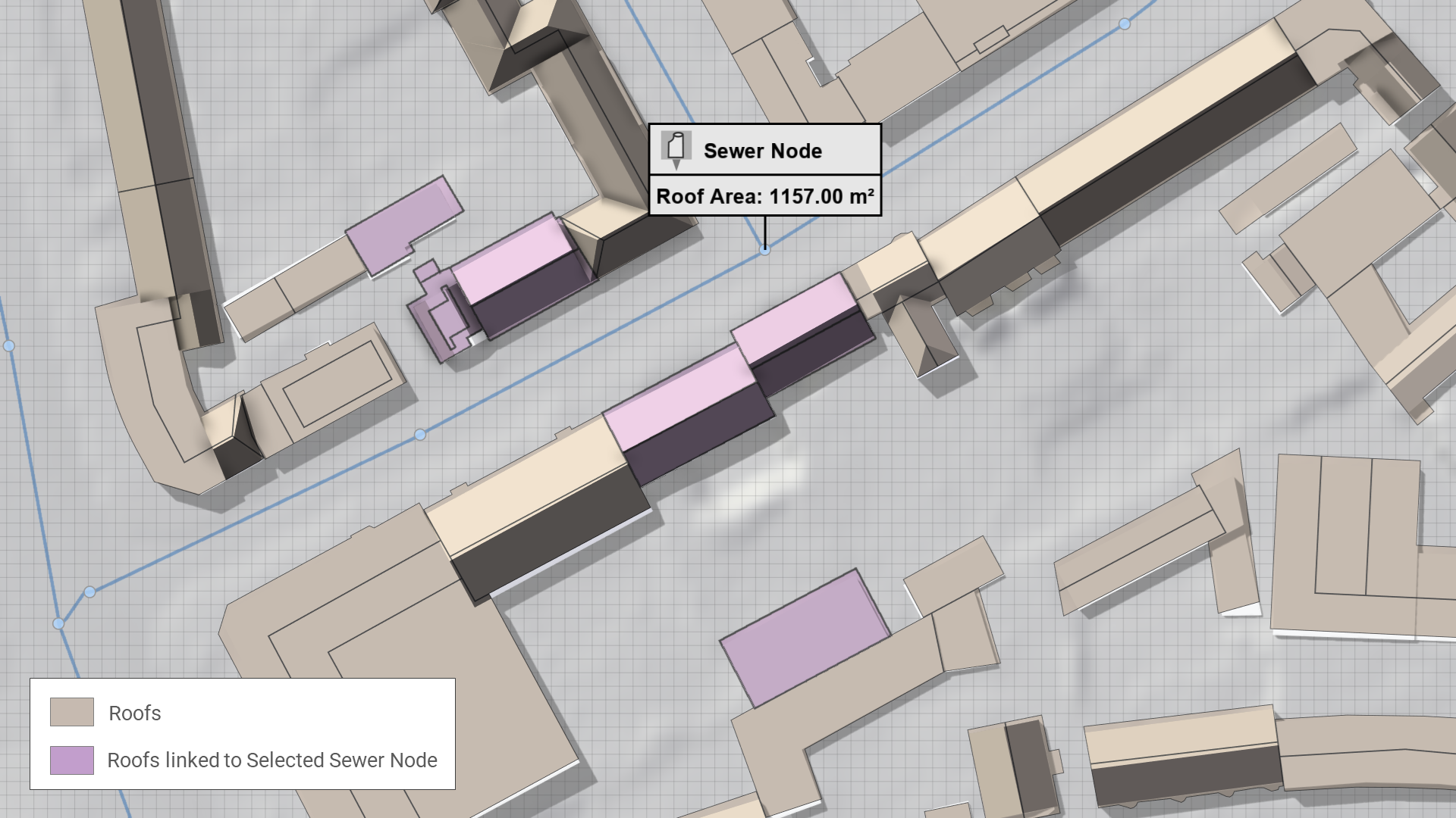
• Roof Polygons:
  This option allows roofs to be loaded from a dedicated shape file. Roof polygons must overlap with a building footprint polygon. A one-to-one or many-to-one relationship between roofs and buildings can be established (e.g., multiple roof polygons for a single building). Additionally, this mode allows specifying attributes such as where the roof water should be redirected, including the option to direct it to specific sewer nodes:
  

Rain

Setup Location: Simulation Settings Panel > Surface: Rain

scenarify offers several options to define rainfall input for your simulation model. These range from simple uniform rainfall to advanced, spatially distributed precipitation from real measurements.

Hint: Test all rain specification methods using the NRW base model from the Quick Start Tutorial.
Example datasets for rainfall are available for download here or directly via the file selector under taskBasedWorkflows/nrw cologne.
The spatially varying dataset comes from a real radar-recorded rain event in Cologne.
Use Address Search with "Duennwald Koeln" to jump to a good test area. Step-by-step instructions follow below.

Spatially Uniform Rainfall

For quick setups, you can define a uniform rain event across the entire simulation domain:

• Enter Rate: Specify a constant rainfall intensity (e.g., 35 mm/h).
• Enter Amount: Define the total rainfall amount applied as a block rain event.

Rain Choice: From KOSTRA (Germany Only)

For models located in Germany, scenarify supports automatic rain generation using KOSTRA data:

• Select Rain Choice: From KOSTRA.
• Choose the return period (e.g., 30-year or 100-year event) or the SRI index (Starkregenindex).
• Define the temporal profile using Precipitation Type (e.g., Block Rain or Euler Type II).

The system then generates a spatially distributed rain event tailored to your simulation domain.

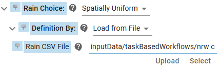
Rain Choice: Spatially Uniform with Load from File

Upload measured precipitation data from a single gauge using a CSV file. You can provide the data either as depth increments or as rain rates over time.

Precipitation Depth IncrementsPrecipitation Rates

Time<time>[];Precipitation Depths<float>[mm]
2010-01-01 00:00:00;0.0
2010-01-01 00:05:00;6.0
2010-01-01 00:10:00;2.0
...

Time<double>[s];Precipitation Rates<float>[mm/h]
0;72.0
300;24.0
600;0.0
...

See the CSV Format Guide for a complete list of supported data types and units.

An example dataset is available for download here (subdirectory: rain data from gauge measurement).

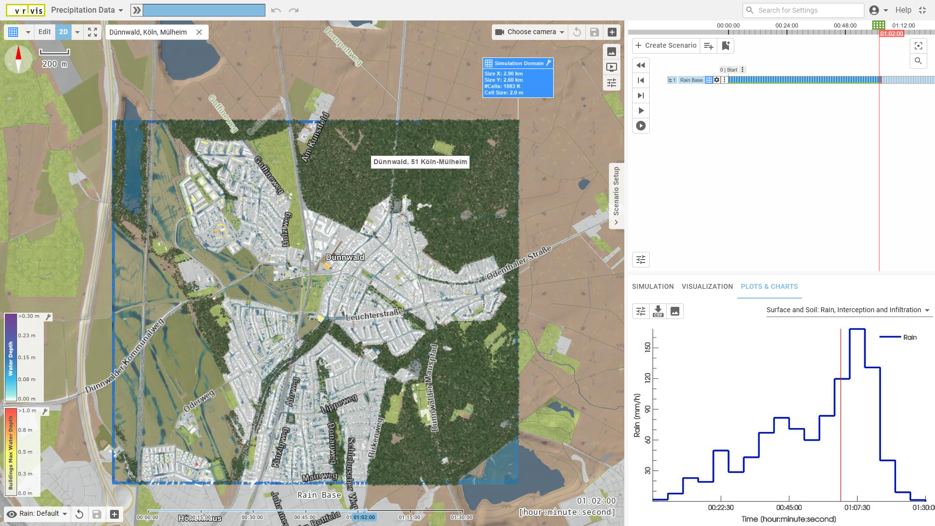
Steps to explore the provided example CSV data

• Create a new project based on New NRW and define a Simulation Domain in Cologne. Use the Address Search and enter "Duennwald Koeln" to quickly find the appropriate area.
• In Simulation Settings Panel > Surface: Rain, change Rain Choice to Spatially Uniform
• Change Definition By to Load from File.
• Select the CSV file from path taskBasedWorkflows/nrw cologne/rain from gauge measurement/rain_event.csv

• Open Plots & Charts > Surface and Soil: Interception and Infiltration to view the loaded rain time series. Make sure the End Time of the active scenario is set to at least 1 hour and 30 minutes to fully cover the rain event duration. The setup is now ready for simulation.

Rain Choice: From Rasters

This option allows you to upload spatially distributed rainfall data over time using a sequence of raster files. Each file represents a single time step and must include a recognizable timestamp in its filename (e.g., rain_2020-05-01_14-00.tif).

This method is ideal for:

• Radar-based precipitation measurements
• Pre-processed effective precipitation inputs, where factors such as infiltration or interception have already been accounted for

Select a directory to load a time series of precipitation raster data. Each time step is stored as a separate raster file. The raster values represent precipitation depth increments, i.e, the rain depth per cell accumulated since the last time step.

scenarify automatically determines the correct simulation time step for each raster based on its file name. Example file names and their interpreted time steps:

Example File Name	Interpreted Time Step
rain_2023-11-05-14-30.tif	5th Nov 2023, 14:30
rain_05-11-2023-14-30.tif	5th Nov 2023, 14:30
rain_14-30.tif	14 hours, 30 minutes after start
rain_60.tif	60 minutes after start

Rules

• Each raster file should represent a single time step of precipitation depths
• The time step size must be constant across all files, e.g., always 5 min between one file to the next.
• If no time pattern is found in the file name, the file will not be placed in the time series.
• Files should be named consistently for correct ordering in the simulation.

Hint: If you plan to use OAK files provided by the state of Baden-Württemberg, Germany, make sure to remove the SUM raster file from the directory before uploading the time step rasters.
This summary file typically has a name like: OAK_AUS_V_1HSUM.tif and can interfere with correct time parsing.

An example dataset is available for download here (subdirectory: rain radar data/from rasters).

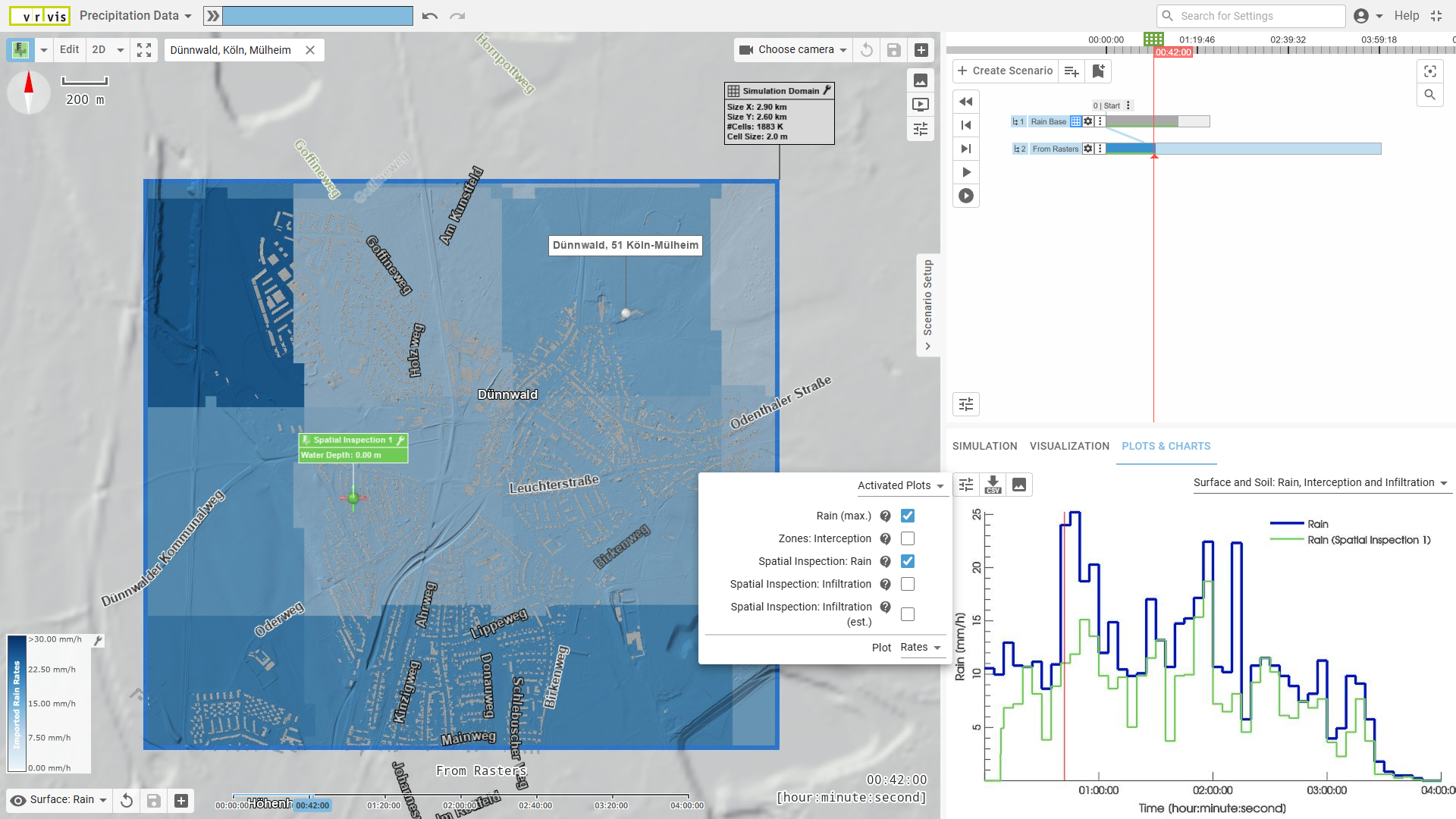
Steps to Explore the Provided Example Radar Data as Rasters

• Begin with the previous steps about exploring the example CSV rain data.
• Create a new scenario and name it "From Rasters". Set the End Time of the scenario to 4 hours to cover the full duration of the radar-recorded event.
• In Simulation Settings Panel > Surface: Rain, change Rain Choice to From Rasters.
• Select the directory containing the raster time series:
  taskBasedWorkflows/nrw cologne/rain radar data/from rasters
• Change the Visual Preset in the View to Surface: Rain. This visualizes the effective rain rates (accounting for interception, walls, etc.) as colored terrain.
• To visualize the imported rain rates only, go to Visualization Settings Panel > Layers: Visualization > Row Terrain and choose:
  Surface: Rain Rate: Imported
• Use the time navigation controls to observe how rain intensity evolves across time and space.
• Open Plots & Charts > Surface and Soil: Interception and Infiltration to monitor the maximum rain rate within the simulation domain.
  To inspect rain at a specific location, use the Spatial Inspection tool.
  Then, in the plot's settings panel, enable Spatial Inspection: Rain to display the time series for that location.

Rain Choice: From Shape and CSV

This option provides an alternative way to define spatially distributed precipitation over time by combining a polygon shape file with a corresponding CSV time series.

Each polygon in the shape file represents an area with unique rainfall data. The CSV file contains time series columns, where each column name must match a polygon attribute (e.g., an ID or name) defined in the shape file. This attribute must be specified in the settings to establish the correct correspondence.

See the example dataset available for download here (subdirectory: rain radar data/from shape and csv).

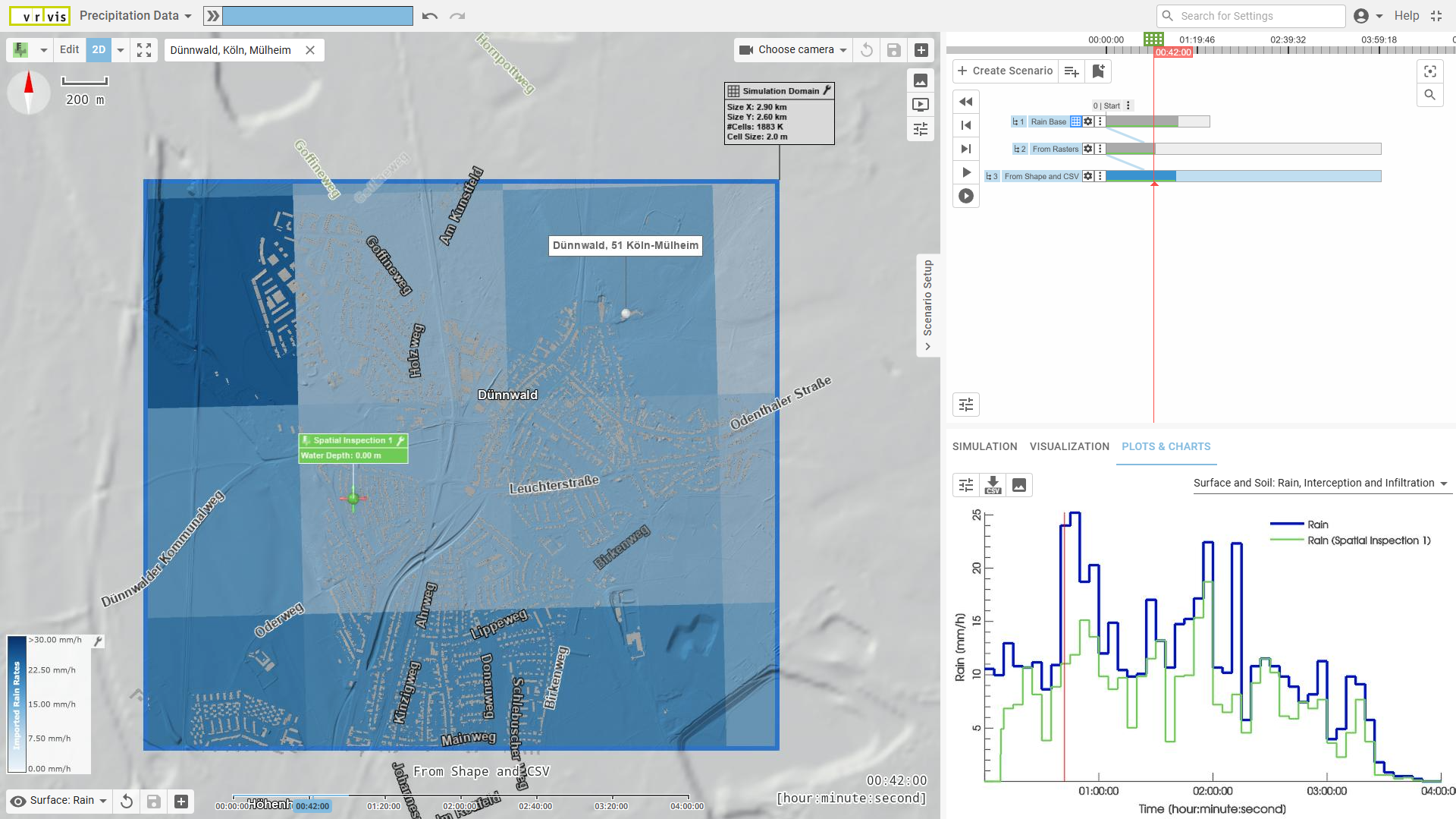
Steps to Explore the Provided Example Radar Data as Shape File and CSV File

• Start by following the previous steps on using radar data as rasters.
  (The shape and CSV example represents the same rain event over Cologne.)
• Create a new scenario based on the "From Rasters" scenario and name it "From Shape and CSV".
• In Simulation Settings Panel > Surface: Rain, change Rain Choice to From Shape and CSV.
• For Rain Increment Depths CSV, select:
  taskBasedWorkflows/nrw cologne/rain radar data/from shape and csv/Radolan_Cologne.csv
• For Rain Shape File (Polygons), select:
  taskBasedWorkflows/nrw cologne/rain radar data/from shape and csv/radolean.shp
• Compare the scenarios "From Rasters" and "From Shape and CSV" to see how the same rain event is modelled with different data sources.

Further Data for Model Details

Setting up these model components does not require any particular order:

Model Data	Purpose	Setup Location
Culverts	Directs water flow beneath roads, railways, or similar structures through pipes or tunnels	Load Actions from File for Culvert
Walls	Represents overtoppable, linear structures that are not depicted in the terrain data	Load Actions from File for Concrete Wall
Bridges	Identifies larger obstacles in terrain data to be removed for flow simulation	Load Actions from File for Structure Removal
Roughness Raster or Polygons	Provides detailed roughness and/or thin-film roughness from raster or shape files, preferred over land use mapping	Simulation Settings Panel > Surface: Roughness
Soil Map	Provides soil type information for infiltration parameter mapping, optionally including measured saturated conductivity values, preferred over land use mapping	Simulation Settings Panel > Soil: Infiltration Zones
Catchments	Supports the definition of simulation domains by catchments and invalidates cells outside the catchment	Simulation Settings Panel > Domain Setup: Catchments
Sink Polygons	Models rivers as sinks in heavy rain simulations to separate heavy rain flood risks from river flood risks	Simulation Settings Panel > Domain Setup: Sink Polygons
River Axis Lines	Facilitates inflow and outflow setups for river flood modeling	Simulation Settings Panel > Rivers and Streams: Axis Lines, see also: River Modeling
River Bank Lines	Facilitates inflow and outflow setups for river flood modeling	Simulation Settings Panel > Rivers and Streams: River Banks, see also: River Modeling
Sewer Network	Enables coupled sewer-surface modeling	Simulation Settings Panel > Sewer Nodes, Sewer Links, and Sewers, see also: Sewer Network Setups