Bidirectional Surface–Sewer Coupling
In urban flood modeling, simulating the interaction between surface water and sewer networks is crucial. The sections below outline the methodology for modeling these exchanges with surface–sewer discharge exchange term depending on the flow conditions. The approach involves coupling surface and sewer models through data exchange and synchronization at pre-defined coupling time steps, ensuring efficient and accurate flood simulations.
Vertical Discharge Exchange
The surface–sewer discharge exchange term depends on the water level at the surface \( w \), the hydraulic head \( H \) at the manhole or storm drain, and the bed surface elevation \( b \). In the following, the area and diameter of the manhole or storm drain are abbreviated with \( A_m \) and \( D_m \), respectively, and \( d_i \) is the distance between the surface and the invert level of the pipes entering the node. The invert level refers to the lowest elevation admitting water flow.
Based on the work of Djordjevic et al. (2005) and Rubinato et al. (2017), four cases are distinguished:
- Inflow into a non-pressurized node.
- Inflow into a pressurized node with small surface flow depth relative to node width.
- Inflow into a pressurized node with large surface flow depth relative to node width.
- Outflow onto the floodplain.
If the head in the pipe network is lower than the surface elevation, i.e., \( H < d_i \), the discharge exchange \( Q_e \) (m³/s) is given by the free weir equation:
If the head in the pipe network exceeds the surface elevation, i.e., \( H > d_i \), the discharge exchange is given by the submerged weir equation if \( h < \frac{A_m}{\pi D_m} \):
If \( h \geq \frac{A_m}{\pi D_m} \) and still \( H > d_i \) holds, the node is considered fully submerged, and thus the submerged orifice equation is considered a more appropriate description:
For circular manholes, the orifice equation is applied if \( h > \frac{D_m}{4} \). The discharge coefficients for the free weir, the submerged weir, and the orifice equations are set to \( c_{d,w} = 0.56 \), \( c_{d,sw} = 0.11 \), and \( c_{d,o} = 0.2 \), respectively, see Rubinato et al. (2017). The specific sewer exchange term for the surface model is limited by the available water on the surface in the case of sewer inflow.
If the head in the pipe system exceeds the water level of the surface flow, an orifice equation is used. Assuming that the surface velocity is negligible, the discharge exchange is given by:
This equation also holds for dry surface cells, i.e., when \( h = 0 \).
With these four cases, all exchange flow conditions are properly handled.
Sewer overflow also occurs if water flow from the roofs of the surrounding buildings exceeds the sewer inflow capacity, see also the page on Roof Water. Consequently, water spills over at this node. In this case, the roof water is directly added to the sewer overflow as excess discharges and not reduced by the surface–sewer exchange equations.
Horizontal Discharge Exchange
At outfalls, the surface water level is prescribed as head for the outfall in the sewer network simulation. Then, the outfall discharge is computed within the sewer network simulation by accounting for the prescribed outfall head. Subsequently, the outfall discharge is then applied both within the sewer network and surface simulation, by removing the corresponding water from the sewer node and adding it to the surface water at the outfall cell.
When backflow from outfalls is activated, water may also enter from the surface into the sewer network at outfalls. In this case, again the surface water level is prescribed as head for the outfall in the sewer network simulation and the backflow discharge is calculated by the sewer network simulation. At the surface, a non-negative surface water depth is ensured by restricting the volume to be removed if it exceeds the available water volume.
Hint: The outfall discharge can be visualized at the outfall nodes and on the terrain. If the outfall discharge is negative, this indicates backflow from the surface into the sewer network.
Spatial Discretization
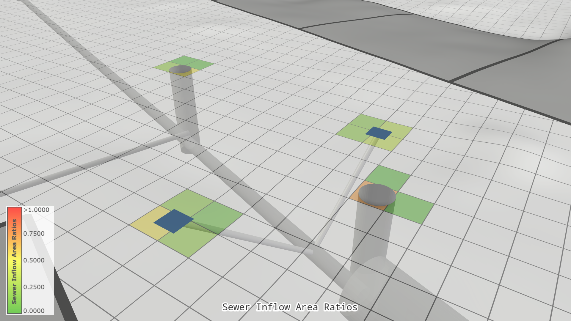
The surface–sewer coupling takes place only at the cells where manholes, storm drains or outfalls are connected to the surface.
To this end, the geometry of the manholes and storm drains is rasterized on the simulation grid. Effectively, at each cell the perimeters and areas of all intersecting manholes and storm drains are collected, resulting in inflow and overflow area ratios per surface cell. The inflow and overflow area ratios already take into account, whether the manhole or storm drain is enabled as an overflow or inflow location in the respective settings.

Furthermore, contributions of each cell to each sewer node are collected. All in all, cases where multiple manholes intersect the same cell, as well as cases where multiple cells contribute to the same node are resolved. For each surface cell, the corresponding node head is found by averaging over all nodes connected to the specified cell. The sewer node exchange discharges are computed on a per-cell basis and totals are given as weighted sums by accounting for the relative contributions.
For outfalls, only the cell located at the outfall position is considered. Also multiple outfalls in a single cell are resolved properly.
Temporal Discretization
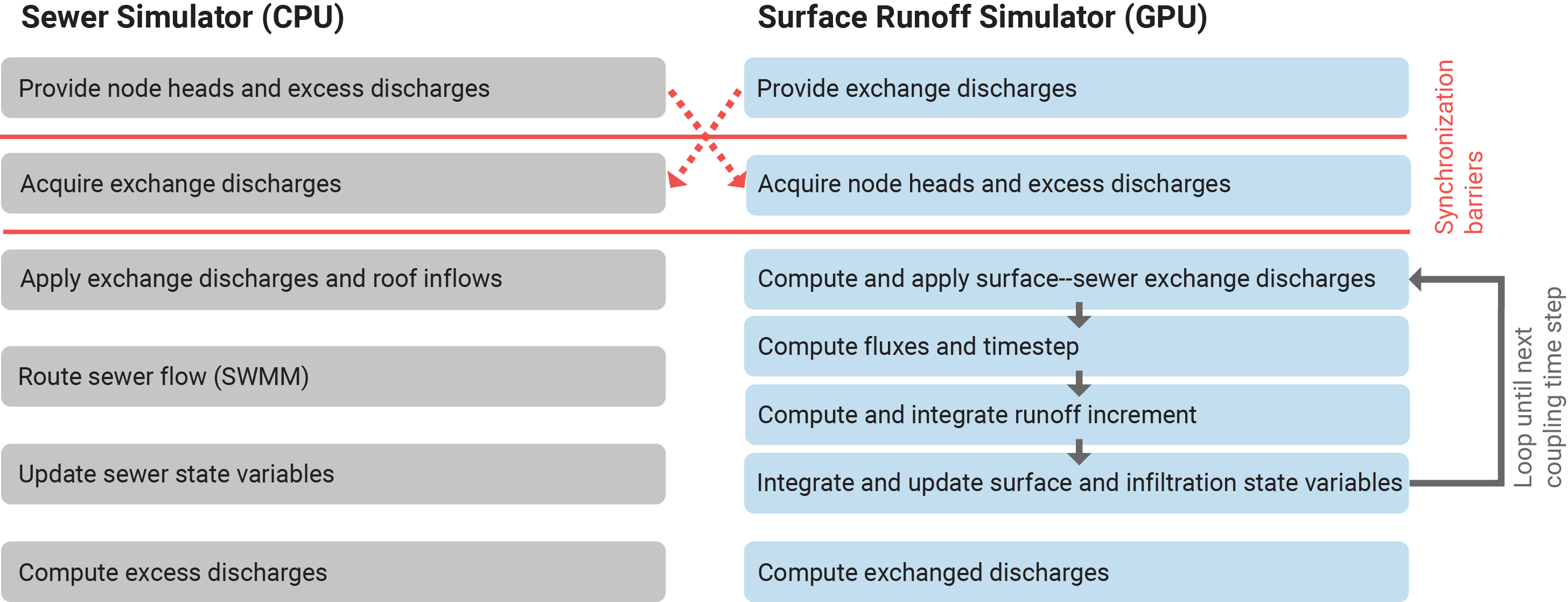
The sewer and surface simulators run in parallel but synchronize for data exchange. These synchronization barriers are necessary for data exchange between the two simulators. With this loosely coupled approach, each simulator advances independently within the coupled model time step. This is summarized in the following diagram:

The sewer network model is interleaved with the surface and runoff model using a pre-defined coupling timestep \( \Delta T_C \). At multiples of this timestep, data is exchanged between the runoff and sewer models. The coupling timestep size also sets an upper limit for the individual simulators' time steps, usually set to 1 second. Typically, the coupling timestep should be similar in size to the individual solvers' timesteps. A coupled model time step is divided into:
- Exchange sewer–surface coupling data (node heads and excess discharges for surface flow, exchange discharges \( Q_e \) for the sewer model).
- Advance the simulators in parallel from the beginning to the end of an coupling time step.
- Compute exchanged discharges for this coupling time step in each simulator.
Each simulator performs multiple routines at each step. When data needs to be exchanged, simulators wait at synchronization barriers, set only at the beginning of a coupled simulation time step. The loop for time steps in the advance step runs independently in each simulator. Each simulator uses the minimal time steps necessary for its numerical stability to advance from the beginning to the end of an coupling time step.
In the sewer simulation, exchange discharges from the surface simulation are applied to the sewer network. Additional inflows, e.g. Roof Water from roofs, are applied and compared with the sewer network's inflow capacities. These excess discharges contribute to node overflow. SWMM routes the Sewer Network Flow, updates the sewer network state, and the excess volumes accumulated during one coupling time step. They are then provided to the surface runoff simulation in the next coupling time step. Thus, the excess discharges that are applied in the surface simulation come from the excess volumes in the sewer network from the previous coupling time step. During the coupling time step, the state of the surface variables remains fixed for the sewer simulation and vice versa.
For the Surface Flow simulation, node heads from the sewer simulation are needed for computing surface–sewer exchange discharges. Once obtained, the surface runoff simulation advances independently. The routines in the surface runoff are looped until the end of the coupling time step. Surface state variables (water depth, level, surface flow discharges) and infiltration state variables are updated after every surface simulation timestep. After the loop, applied exchange discharges are computed and provided to the sewer simulation in the next coupling time step.
The coupled simulation time steps continue until the simulation end time is reached. As the sewer and surface runoff simulations run in parallel, the execution time of the coupled model is determined by the slower simulator, not by the sum of their execution times. Typically, the one-dimensional sewer network simulation is faster than the two-dimensional surface flow simulation, though the sewer simulation can become a limiting factor for very large sewer networks (e.g., over 20,000 nodes).
For more details, see Buttinger et al. (2022).
References
Buttinger-Kreuzhuber, A., Konev, A., Horváth, Z., Cornel, D., Schwerdorf, I., Blöschl, G., and Waser, J., 2022. An integrated GPU-accelerated modeling framework for high-resolution simulations of rural and urban flash floods. Environ. Modell. Softw. 105480.
DOI: 10.1016/j.envsoft.2022.105480
Djordjević, S., Prodanović, D., Maksimović, Č., Ivetić, M., and Savić, D., 2005. SIPSON – simulation of interaction between pipe flow and surface overland flow in networks. Water Sci. Technol. 52 (5), 275–283.
DOI: 10.2166/wst.2005.0143
Rubinato, M., Martins, R., Kesserwani, G., Leandro, J., Djordjević, S., and Shucksmith, J., 2017. Experimental calibration and validation of sewer/surface flow exchange
equations in steady and unsteady flow conditions. J. Hydrol. 552, 421–432.
DOI: 10.1016/j.jhydrol.2017.06.024