Hydrodynamic Simulation Model
Imagine a raindrop's journey as it falls from the sky, becoming part of a detailed simulation. It starts with precipitation, where our model accurately tracks rain volumes. Some droplets are intercepted by vegetation, captured before reaching the ground, with the model accounting for various plant types and canopy structures. As the raindrop hits the ground, some of it becomes surface runoff, flowing over the land. This runoff then flows into streams, with the model considering terrain and vegetation to predict surface water flow and stream discharges. A portion of the surface runoff infiltrates the soil, with rates depending on soil type and moisture levels. In urban areas, part of the rainwater lands on rooftops and might be held back in green roofs. Excess roof water and surface runoff may enter drainage systems and sewer networks, crucial for managing stormwater in cities. This journey, meticulously followed by our hydrodynamic simulation model, provides invaluable insights for managing water resources and flood risks.
Overview of Model Components
In essence, scenarify's coupled 1D/2D hydrodynamic simulation tracks a raindrop's journey through the following processes:
-
- Precipitation
- Interception
- Roof Water
- Infiltration
- River Inflows and Outflows
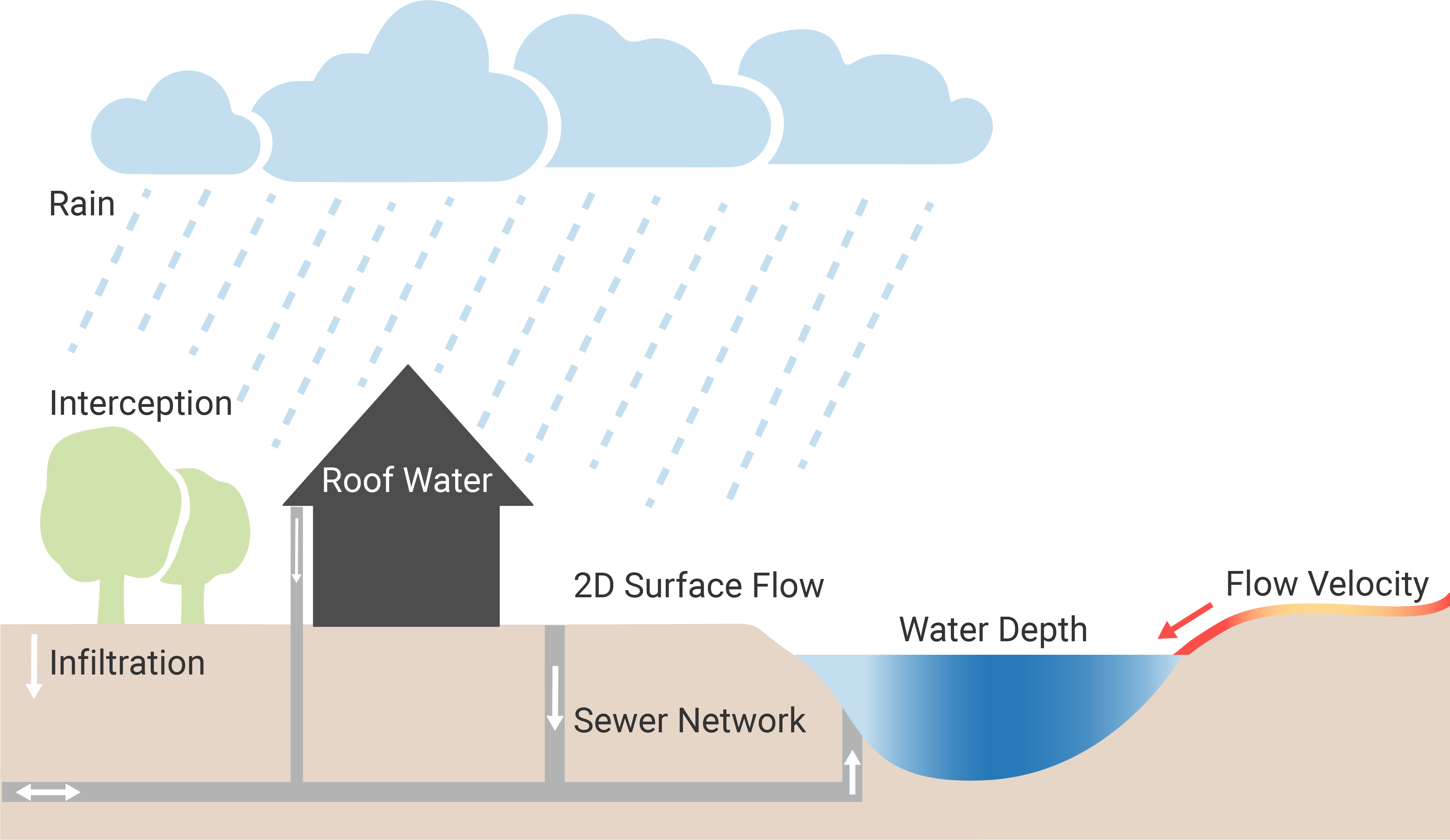
In scenarify, all these components are incorporated as one integrated, time-dependent coupled model, where changes in one submodel are immediately reflected in others during each simulation time step.
Hydrology
scenarify inherently integrates essential hydrological parameters to meet the requirements of model-based urban flood prevention. Detailed descriptions of how hydrological rainfall-runoff modeling is incorporated are provided in the following sections.
Rain may be specified in a spatially uniform or in a spatially distributed way, for example from rain radar raster data. The prescribed precipitation rates are then reduced by specified interception loss rates, resulting in effective precipitation rates. Effective precipitation is modeled as a source term in the 2D shallow water equations.
Traditionally, watershed polygons and hydrological balance equations are used to calculate effective runoff. In scenarify, runoff is computed through raster-based hydrodynamics, also called rain-on-grid approach, accounting for losses due to infiltration and interception using the same equations as traditional rainfall-runoff modeling on a per-cell basis.
Interception losses are considered through a constant loss rate that reduces local rainfall based on the prevailing land use on a cell-by-cell basis. This reduction is effective at the beginning of a heavy rainfall event until the interception storage is filled. The interception storage capacity is parameterized according to land use. Empirical values from the literature are utilized in the standard parameterization.
Soil absorbs surface water at the current infiltration rate until the wetting front depth exceeds the soil thickness. In each cell, these infiltration rates are calculated using the Green–Ampt model. This semi-physical approach considers the ponding height of surface water and the three infiltration parameters:
- the saturated hydraulic conductivity,
- the suction head along the wetting front
- the moisture deficit (or soil moisture).
The infiltration parameters are set using soil maps. Additionally, impermeable surfaces, e.g. paved areas, are considered, there no infiltration occurs.
Rivers and streams are accounted for by specifying river inflows and outflows where rivers enter or leave the simulation domain.
Roof water generated by runoff from building roofs is split according to the current settings. Excess roof water from roofs not connected to the sewer system is distributed onto the surrounding valid cells of the 2D simulation domain. Roofs connected to the sewer system drain into the corresponding node of the sewer network model.
Nature-based solutions, e.g. green roofs, are modeled as a multi-layer system. They may feature a crust layer, a soil layer and a storage layer. Additionally, a constant loss rate can be set.
2D Hydrodynamic Surface Model
The surface water simulation in scenarify uses a state-of-the-art solver for the two-dimensional (2D) shallow water equations. The equations are discretized using an explicit finite volume method on a structured rectangular grid. The temporal discretization is given by the maximum simulation time step computed from the CFL condition. Spatially distributed friction is calculated with the Gauckler-Manning-Strickler formula by specifying roughness parameters according to land use. The surface water simulation has been extensively validated through analytical solutions, laboratory experiments, and historical events.
Water bodies and open stormwater retention basins are modeled on the 2D level using the surface model. An inital state can be assigned in several ways, ranging from GeoTIFF files to initial state propagation from user-defined actions.
Culverts are available to simulate confined water flow beneath the surface, e.g. under a road, railroad, building. Structures which are representable in the terrain, e.g. weirs, levees, or retention basins, are directly incorporated into scenarify's 2D surface water model. scenarify enables interactive terrain adjustments to enable on-the-fly planning or fast model setup in the case of incomplete digital data.
Various barrier types are supported in scenarify, which are typically used to protect important objects. However, these protection measures might fail, leading to severe consequences. Such what-if scenarios can be explored and quantified in scenarify.
Wall boundaries are used to represent impermeable building walls. Moreover, the base areas of buildings are cut out of the computational grid of the surface model, preventing them from being flooded at any time.
Sewer Network Model
The SWMM model is integrated into scenarify for sewer network simulation, encompassing various sewer structures such as weirs, storage, and pumps. The solver for the one-dimensional (1D) hydrodynamic sewer network simulation is using an implicit finite difference method.
Surface–Sewer Coupling
The bidirectional coupling between surface and sewer network allows the dynamic exchange of water at each simulation time step. Water volume can be transferred from the sewer network to the surface model in the form of manhole overflow. Conversely, water from the surface can enter the sewer through storm drains and manholes if there is available capacity. Mathematically, the bidirectional surface–sewer coupling of the models is achieved through the (flooded) weir or orifice equation, with an additional upper limit on the inflow capacity into the sewer network. Furthermore, there is horizontal bidirectional coupling at the inlet and outlet structures of the sewer network with water bodies to simulate complex interactions there.