From MIKE

Tutorial 2: Shape Files Derived from a MIKE URBAN Model

This tutorial covers a sewer network model for the same domain as the previous one, but the shape files used here have been derived from a MIKE URBAN model. While the basic setup principles remain the same, the key differences lie in how the attribute tables are configured, due to different attribute naming conventions. As a result, this tutorial focuses primarily on setting up the attribute tables. We strongly recommend reviewing the previous tutorial first, as it introduces all the foundational concepts.

The .zip archive containing the sewer network shape files for this tutorial is available for download here. When selecting shape files in the Simulation Settings Panel, there is no need to re-upload the data. All files are already accessible by navigating to: Input/taskBasedWorkflows/denmark/sewers/fromMIKE.

0. Model area and scenario

This step repeats the corresponding step of Tutorial 1.

1. Junctions

Setup location: Simulation Settings Panel > Sewer Nodes: Junctions or All

In the Shape File (Points) field, choose the file MIKE_nodes.shp from the example data provided in the link above. Set up the attribute table as follows:

Setup 1

If the junctions are set up fine, the visual results in the View will resemble those from the corresponding step of Tutorial 1.

2. Outfalls

Setup location: Simulation Settings Panel > Sewer Nodes: Outfalls

In the Shape File (Points) field, select the file MIKE_outlets.shp from the example data linked above. Configure the attribute table as shown below:

Setup 2

If the outfalls are configured correctly, the visual results in the View will resemble those from the corresponding step of Tutorial 1.

3. Storages

Setup location: Simulation Settings Panel > Sewer Nodes: Storages

In the Shape File (Points) field, choose the file MIKE_basins.shp from the example data referenced above. Specify the attribute names in the attribute table to load the storage units into scenarify:

Setup 3

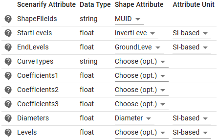
In the Custom Storage Profiles File Path field, select the file storage_profiles.csv included with the dataset. The results in the View should resemble those from the respective step of Tutorial 1.

Hint: In this example, the CurveTypes in the attribute table remain unset ("Choose (opt.)") because scenarify automatically searches the storage profiles .csv file for all storage IDs and assigns the TABULAR curve type to those found.

4. Conduits

Setup location: Simulation Settings Panel > Sewer Links: Conduits

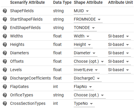
In the shape file selection field Shape File (Lines), select the file MIKE_links.shp to load the conduits. Set up the attribute table as follows:

Setup 4

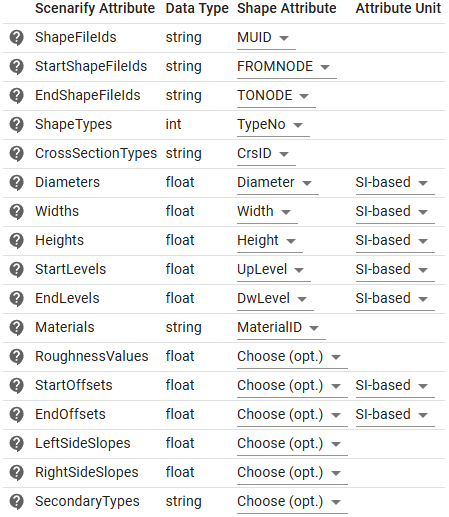
Under Custom Cross-Section Profiles, in the CSV File Path field, select the file conduit_profiles.csv provided with the dataset. Ensure that the Scale Custom Profile Dimensions by Link Height checkbox is enabled — for more context, refer to the corresponding step in Tutorial 1.

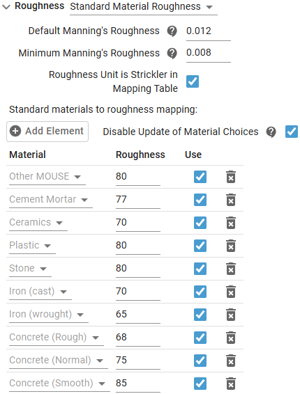
In the attribute table, the "Materials" field specifies material names for each conduit, which determine the conduit roughness. The mapping from material names to roughness values is handled in scenarify under the Roughness section via "Standard Material Roughness". This predefined mapping already covers all materials in the example shape file except one: "Other MOUSE". To address this, we extended the mapping by clicking "Add Element" and assigning "Other MOUSE" a generic roughness value of 80 (Strickler scale):

Setup 5

If the conduits are set up correctly, the results in the View will resemble those from the corresponding step of Tutorial 1.

5. Weirs

Setup location: Simulation Settings Panel > Sewer Links: Weirs

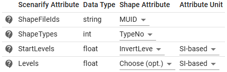
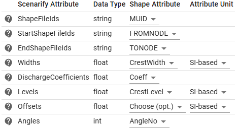
Under Shape File (Lines or Points), select the file MIKE_weirs.shp from the example data provided in the link above and configure the attribute table:

Setup 6

Refer to step 5 in Tutorial 1 to compare the results in the View—they should appear similar.

6. Pumps

Setup location: Simulation Settings Panel > Sewer Links: Pumps

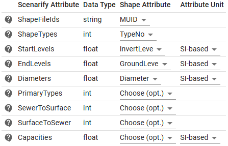
In order to load pumps, select the file MIKE_pumps.shp in the corresponding Shape File (Lines or Points) field. The attribute table should be configured the following way:

Setup 7

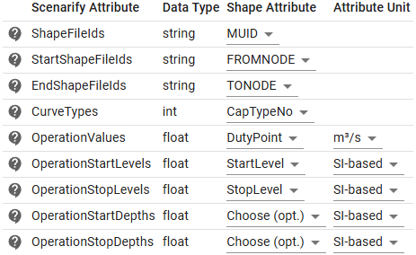
Pumps can be characterized by their operation mode (see "CurveTypes" in the attribute table) and maximum capacity. In scenarify, the maximum capacity attribute name is set under OperationValues in the attribute table. Some datasets express pump capacities in m³/s, while others use l/s. Be sure to verify the units in your dataset and specify them in the Attribute Unit column if necessary.

If the pumps are set up correctly, the visual results in the View will resemble those from the corresponding step of Tutorial 1.

7. Orifices

Setup location: Simulation Settings Panel > Sewer Links: Orifices

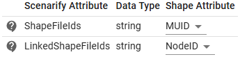
In the Shape File (Lines or Points) field, choose the file MIKE_orifices.shp from the example data referenced above to load the orifices into scenarify. Set the attribute table as follows:

Setup 8

The results in the View should resemble those from the respective step of Tutorial 1.

8. Catchments

Setup location: Simulation Settings Panel > Sewers: Catchments

Load the file MIKE_catchments.shp in the corresponding field Shape File (Polygons). The attribute table should be configured as in the figure below:

Setup 9

As in the corresponding step of Tutorial 1, catchments should become visible when using the Sewer Node Inspection action with the option to display associated node catchments enabled.

9. Simulation settings

Setup location: Simulation Settings Panel > Sewers: Simulation Model, Simulation Settings Panel > Buildings: Roofs

This step repeats the corresponding step of Tutorial 1.

Hint: If configured properly, the resulting scenario will match the "Sewers Bellinge Base (MIKE)" scenario available in all projects derived from the Denmark base model.