From SWMM

Tutorial 1: Shape Files Derived from a SWMM Model

The .zip archive containing the sewer network shape files used in this tutorial is available for download here. When selecting shape files in the Simulation Settings Panel, there is no need to re-upload the data. All files are already accessible by navigating to: Input/taskBasedWorkflows/denmark/sewers/fromSWMM.

0. Model area and scenario

Create a new project using the Denmark base model (New > New Denmark). This model, built from open-source data, is available for trial use by all users. In the project, use the Address Search feature to locate Bellinge. Create a new scenario and place the simulation domain around Bellinge:

1. Junctions

Setup location: Simulation Settings Panel > Sewer Nodes: Junctions or All

In the Shape File (Points) field, choose the file SWMM_nodes.shp from the example data provided in the link above. Upon loading the shape file, scenarify will automatically switch to Edit Mode.

Hint: When loading a shape file for the first time, you might need to click the Run button to force scenarify to parse it once and update the possible choices for attribute names.

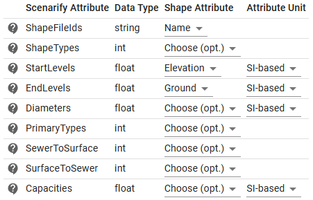
The attribute table contains mandatory attributes marked with "Choose" and optional attributes marked with "Choose (opt.)":

If an attribute is marked as "Choose", you must assign the corresponding shape file attribute name. If it's marked as "Choose (opt.)", assigning it is optional. To intentionally leave out an optional attribute, set it to "Choose (opt.)". If the attribute is required but left unset, the simulation will fail and show an error message. In some cases, at least one of two optional attributes must be specified (for example "Levels" or "Offsets" for weir crests). Therefore, we recommend always consulting the inline helper tooltips when configuring attribute tables. For this tutorial, set up the attribute table as shown below:

After setting up the attribute table, click the Run button to exit Edit Mode. The View should now display the sewer junctions:

Hint: Initially, the loaded sewer data might not be visible. This can happen because the current visual preset does not display sewer elements. Make sure to select a visual preset from the "Sewers" category—such as "Sewers: Default".

2. Outfalls

Setup location: Simulation Settings Panel > Sewer Nodes: Outfalls

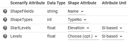
In the Shape File (Points) field, select the file SWMM_outfalls.shp from the example data linked above. Set up the corresponding attribute table as follows:

After clicking the Run button, scenarify will visualize the outfalls as blue circles:

At this stage, since no links (such as conduits, weirs, or pumps) have been defined yet, you can disregard the warnings that say, "Unable to find a link for an outfall." However, once all available sewer network components have been specified, you should carefully review all displayed warnings, as they may indicate missing or incorrect data.

Hint: A complete list of sewer network verification warnings—each linked to the corresponding shape file ID—can be downloaded as a .csv file from the Simulation Settings Panel, under category Sewers: Simulation Model.

3. Storages

Setup location: Simulation Settings Panel > Sewer Nodes: Storages

In the Shape File (Points) field, choose the file SWMM_storages.shp from the example data referenced above to load the storage units into scenarify. Configure the attribute table as follows:

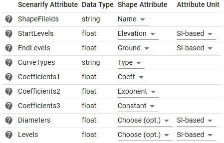
Storage units are designed to temporarily hold excess water during peak periods. Their retention capacity is defined by their volume and shape, typically represented by the relationship between surface area and water depth. This relationship can be described either by a functional formula or through a dedicated .csv file. The description method used for each storage unit is specified by "CurveTypes" in the attribute table:

• If the curve type of a storage unit is FUNCTIONAL, a functional definition is expected. Let \( A \), \( B \), and \( C \) stand for the corresponding values of "Coefficients1", "Coefficients2" and, "Coefficients3", respectively. Then the functional dependency of the storage surface area \( y \) on water depth \( x \) is expressed as \( \; y= A \cdot x^B + C \)
• If the curve type of a storage unit is TABULAR, a tabular definition in a .csv file is expected

For this tutorial, in the CSV File Path field under Storage Profiles, select the file storage_profiles.csv included with the dataset:

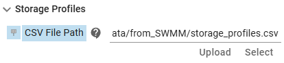
You can scroll through storage_profiles.csv to examine how the relationship between water depth and surface area is defined for individual storage units, identified by their unique IDs. Only storages with the curve type TABULAR are included in this file. For these TABULAR storages, the values in the "Coefficients1", "Coefficients2", and "Coefficients3" fields are ignored.

Hint: If "CurveTypes" are not specified, scenarify defaults to using simple cylindrical storage units based on the provided diameters. A warning message will appear in such cases, indicating that a fallback to cylindrical storage has occurred.

4. Conduits

Setup location: Simulation Settings Panel > Sewer Links: Conduits

In the file selection field, choose the file SWMM_conduits.shp to load the conduits. Set up the attribute table as follows:

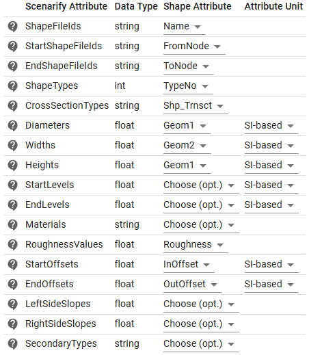
Among other parameters, sewer conduits are characterized by cross-sectional shape. Basic shapes, such as circular or rectangular, can be fully described by attributes like diameter, width, and height. However, for more complex ("custom") cross-sections, a tabular definition is needed, typically provided in a .csv file. Each custom cross-section, identified by a unique cross-section ID ("CrossSectionTypes" in the attribute table), specifies the relationship between height and width at various points along the cross-section. Take a moment to examine the file conduit_profiles.csv before specifying it under Custom Cross-Section Profiles:

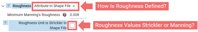
Custom profile descriptions can be specified using either absolute distance units (meters) or normalized values relative to the conduit height. In the example file provided, the height column ranges from 0 to 1, indicating that the profile is given in normalized units. Therefore, you should make sure to activate the corresponding checkbox in scenarify, which instructs the system to scale each custom profile description by the actual conduit height where the profile is applied.

Hint: If custom conduit profiles are not specified or a profile cannot be found for a specific cross-section ID, scenarify will default to circular cross-sections for those conduits lacking custom profile descriptions. To indicate this, a warning message will appear.

Conduit roughness influences how quickly water flows through a conduit. In scenarify, it can be defined either by mapping material names from the "Materials" field or directly via the "RoughnessValues" field in the attribute table. In this tutorial, roughness is specified directly (notice how in the attribute table, "RoughnessValues" are specified and "Materials" are not), so under Roughness, choose "Attribute in Shape File":

Once loaded, you will see that the junctions are now visually connected to each other in the View:

Hint: The bare minimum required for a sewer network simulation includes junctions, conduits, and at least one outfall. These components ensure water flow can be routed through the system, with the outfall serving as the final discharge point for the simulation.

5. Weirs

Setup location: Simulation Settings Panel > Sewer Links: Weirs

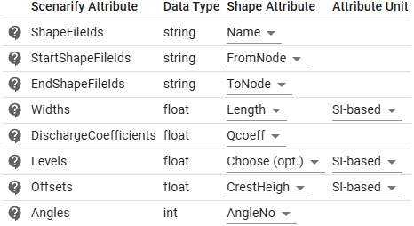
Under Shape File (Lines or Points), select the file SWMM_weirs.shp from the example dataset linked above. Unlike previous file fields, this one accepts both line and point shape files. While sewer links are typically represented as lines, certain modeling tools—such as HYSTEM-EXTRAN—use points to represent special sewer structures like weirs, pumps, or discharge restrictors. In such cases, the structure-specific properties (e.g., weir discharge coefficients or pump curve types) are taken from the corresponding point-based shape file, while geometry and connectivity are derived from the common line-based link shape file using matching IDs. In this tutorial, however, a standard line-based representation for weirs is used.

Set up the attribute table as follows:

After clicking the Run button, the weirs will be displayed as brown lines in the View:

Hint: Currently, only rectangular weirs with either transverse or sideflow crests are supported.

6. Pumps

Setup location: Simulation Settings Panel > Sewer Links: Pumps

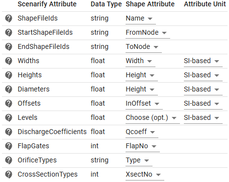
In order to load pumps, select the file SWMM_pumps.shp in the corresponding Shape File (Lines or Points) field and configure the attribute table as shown below:

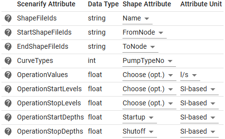
Pumps are link elements used to move water to higher elevations. The relationship between a pump’s flow rate and the hydraulic conditions at its inlet and outlet nodes is defined by a pump curve. scenarify supports five types of pump curves. The curve type for each pump is specified in the attribute table using the "CurveTypes" field. Refer to the inline tooltips for descriptions of the available curve types and the integer codes used to represent them. Further reading on pump curve types can be found in SWMM 5.1 User Manual, page 54.

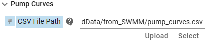
For each pump, in addition to specifying its curve type, the corresponding pump curve must be provided. These curves should be listed in a .csv file, with each entry identified by a pump ID. Under Pump Curves, use the CSV File Path selector to load the file pump_curves.csv from the example dataset linked above:

Take a moment to scroll through the pump_curves.csv file to see how the curves are defined. Note that the argument column is labeled generically as "Argument"—this is intentional, as the interpretation of the argument varies depending on the pump curve type (e.g., inlet node depth, head difference between inlet and outlet nodes, etc.). For every pump that is not defined as an ideal pump, a corresponding pump curve must be provided.

If loaded correctly, the pumps will be visualized as yellow lines in the View:

7. Orifices

Setup location: Simulation Settings Panel > Sewer Links: Orifices

In the Shape File (Lines or Points) field, choose the file SWMM_orifices.shp from the example data referenced above to load the orifices into scenarify. Set up the corresponding attribute table as follows:

In scenarify, orifices are displayed as purple lines:

8. Discharge controllers

Setup location: Simulation Settings Panel > Sewer Links: Discharge Controllers

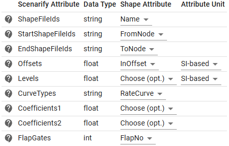
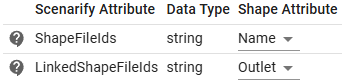
Discharge controllers in scenarify are flow control devices used to model specific depth-discharge or head-discharge relationships that cannot be modelled by pumps, orifices, or weirs. Choose the file SWMM_outlets.shp in the Shape File (Lines) field and set up the attribute table as shown in the image below:

Similarly to pumps, discharge controllers require rating curves to describe how their discharge depends on the conditions at their inlet and outlet nodes. The type of dependency is defined by "CurveTypes" in the attribute table. Possible values include FUNCTIONAL/DEPTH, FUNCTIONAL/HEAD, TABULAR/DEPTH, and TABULAR/HEAD. The DEPTH variant means that discharge depends on the water depth at the inlet node, while the HEAD variant means that discharge depends on the head (absolute water level) difference between the inlet and outlet nodes. The distinction between FUNCTIONAL and TABULAR follows the same principle as for storage units:

• If the curve type of a discharge controller is set to FUNCTIONAL, a functional rating curve must be defined. Let \( A \) and \( B \) represent the values specified in the "Coefficients1" and "Coefficients2" fields, respectively. The discharge \( y \) is then calculated based on the corresponding argument \( x \) (either inlet depth or head difference) using the formula \( \; y= A \cdot x^B \)
• If the curve type of a discharge controller is set to TABULAR, a tabular definition in a .csv file is expected

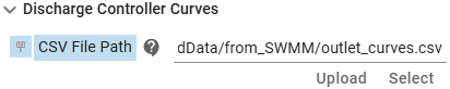
For this tutorial, in the CSV File Path field under Discharge Controller Curves, select the file outlet_curves.csv included with the dataset:

The "Coefficients1" and "Coefficients2" fields are left unset in the attribute table because in this tutorial all discharge controllers in the dataset use the TABULAR curve type.

If loaded successfully, the discharge controllers are visualized as purple lines in the View:

9. Catchments

Setup location: Simulation Settings Panel > Sewers: Catchments

In scenarify, sewer node catchments are utilized for connecting storm drains to sewer conduits (if storm drains are present) and for attributing roof runoff to sewer nodes. To load catchments, select the file SWMM_subcatchments.shp from the provided example data in the Shape File (Polygons) field. The attribute table includes the unique IDs of the catchments and the corresponding unique IDs of the linked sewer nodes. Set it up as follows:

To visualize the loaded sewer catchments, you can utilize the Sewer Node Inspection action and select the option to display the associated catchments. Apply the action to individual sewer nodes to display their associated catchments:

10. Simulation settings

Setup location: Simulation Settings Panel > Sewers: Simulation Model, Simulation Settings Panel > Buildings: Roofs

The sewer network model is now fully set up. As the final step, enable sewer network simulation in the Sewers: Simulation Model category. In Buildings: Roofs, activate roof water management by clicking on Enable Roof Water and set Roof Polygons Choice to "Building Polygons in Sewer Catchments". Once these settings are configured, click on Play scenario in World Lines to initiate the simulation:

Hint: If set up correctly, the resulting scenario should replicate the scenario named "Sewers Bellinge Base (SWMM)", which is included in every project based on the Denmark base model.