Integrating SMS Data
This workflow explains how to integrate SMS 2D mesh data (.2dm) into a scenarify model to enrich it with measured riverbed topography, surface roughness information, and boundary conditions.
While scenarify can import geometry and roughness data directly from .2dm files, boundary conditions are not automatically converted into scenarify’s native format. Instead, this tutorial provides guidelines for manually translating SMS boundary conditions into the corresponding scenarify actions. To support this process, scenarify offers several visual helpers derived from the .2dm file to assist in identifying and configuring boundaries:
- Mesh display – visualize the SMS mesh to inspect thin walls, channel edges, or localized features.
- NodeStrings – display these as lines and labels to understand boundary alignments and parameters.
Boundary information parsing may not cover all SMS formats or versions. See the Supported SMS Tags section at the end for a detailed overview of currently recognized tags and usage notes.
Prerequisites
Before starting, you should be familiar with:
- The scenarify user interface (complete at least the Quick Start Tutorial)
- The Fast Setups with the Setup Wizard Tutorial
- The River Flood Tutorial, which introduces hydrodynamic setups with inflows and outflows.
Example Dataset
This tutorial builds upon the base model of Nordrhein-Westfalen (NRW) in Germany, extending it locally with detailed data for the Godesberger Bach reach. The associated SMS model was provided by Bezirksregierung Köln and can be downloaded here: NRW SMS Example Data
Note: You can also start from a New Blank project and work solely with the SMS data if you prefer, or add your own supplementary data as needed. In our tutorial, we use the NRW base model, as it provides the advantage of an already detailed and well-prepared data foundation.
1. Prepare a New Project and Scenario
- Create a new project from the Project menu by selecting New NRW.
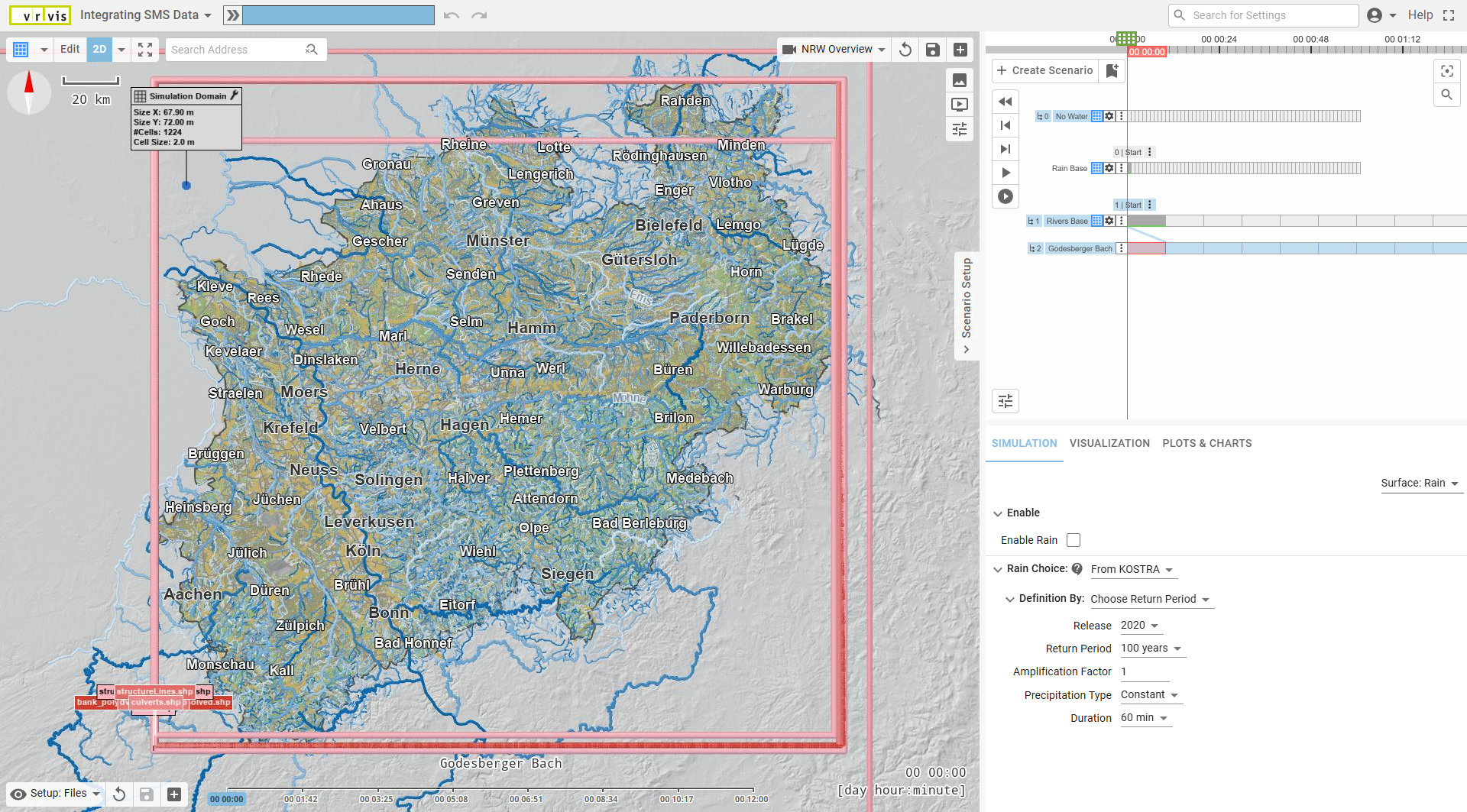
- Open the Scenario Setup Pane and select the bookmark named "Start" of the base scenario "Rivers Base".
- In the bottom-left corner of the View, choose the visual preset Setup: Files.
This preset displays the spatial extents of all files loaded in the model as red bounding boxes.
We will use this visualization to quickly locate the SMS model and to define the simulation domain based on its bounds. - It is recommended not to modify the base scenario directly, for example, if you plan to set up multiple simulation domains within the same project.
Thus, create a new scenario derived from Rivers Base and name it Godesberger Bach.
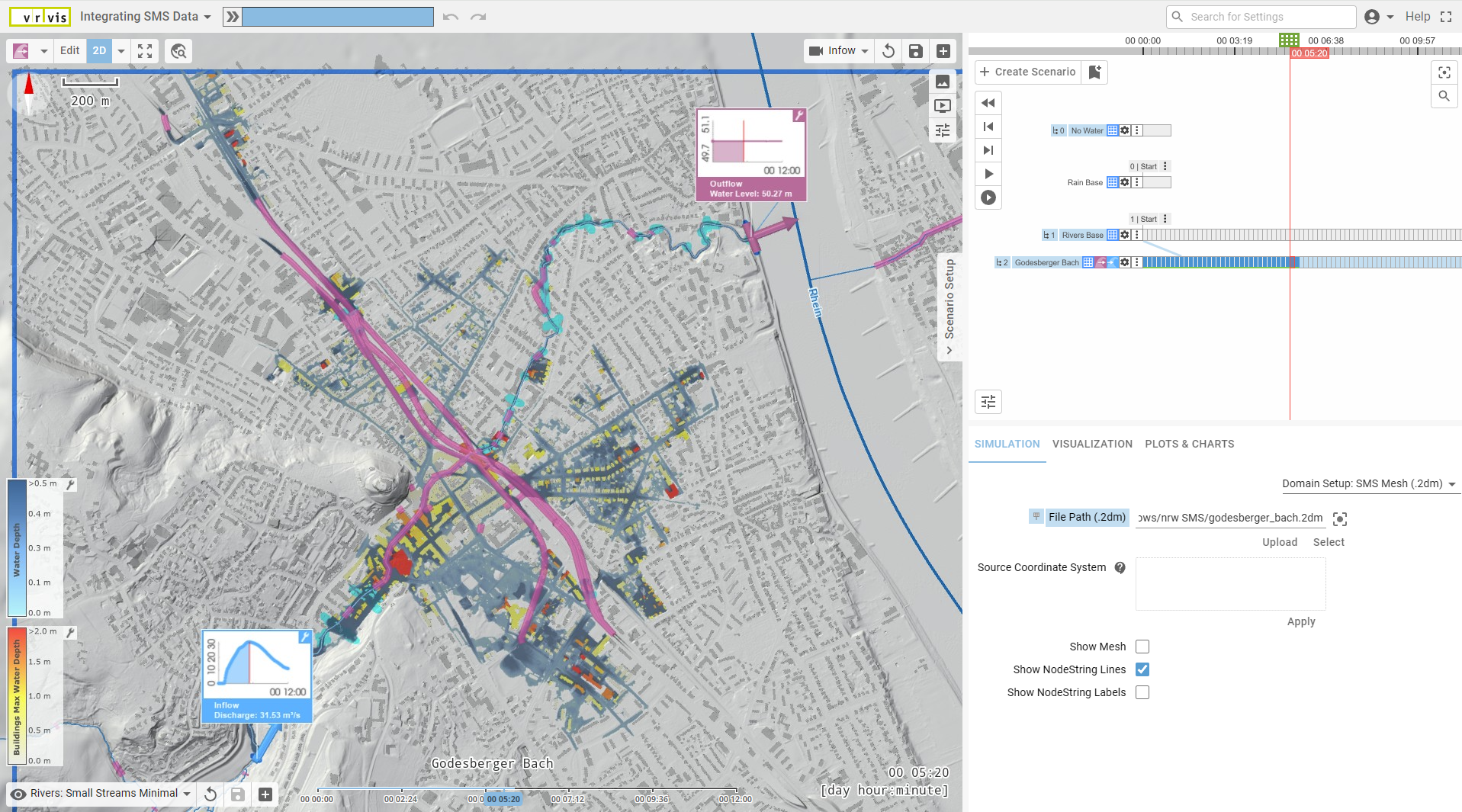
After completing these steps, the View and interface should appear as shown below
2. Import the .2dm File and Define the Simulation Domain
In the Simulation Settings panel, under Domain Setup - SMS Mesh (.2dm), select the path to the example file:
Input/taskBasedWorkflows/nrw_SMS/godesberger_bach.2dm
Note: The Source Coordinate System (CS) of this .2dm file matches the local coordinate system of the NRW base model, so no manual CS entry is needed here. In general, however, you should specify the CS of your SMS data before uploading the file. It is recommended to first enter the CS (e.g., as an EPSG code such as
EPSG:25832in this example) and then upload the .2dm file.
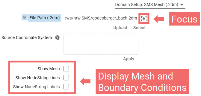
After selecting the .2dm file, click Run to exit Edit Mode and load the data.
The View now displays the spatial bounds of the SMS mesh, and a Focus button appears next to the file selector (see screenshot above). Use this button to center the View on the loaded mesh.
Next, assign the Simulation Domain action to the file bounds by clicking on the boundary line, and set the cell size to 2 m in its Action Settings Panel. Then click Run to load the NRW base model within this domain at the specified resolution.
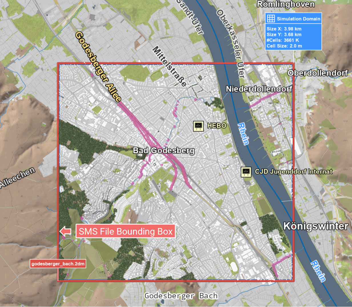
Important: At this stage, nothing from the .2dm file has been used yet.
We have only applied its file bounds to define the simulation domain. All data within the domain, including the terrain, still comes from the base model. We will first use the base model as is to set up a river flood simulation and later gradually integrate more structural details from the .2dm file.
3. Setup Inflows and Outflows
Next, we will use contextual information from the SMS data to locate the inflow and outflow boundaries.
In the View, select the visual preset Rivers: Small Streams Minimal. This preset provides suitable water visualization settings for rivers of this scale and reduces visual clutter, making it easier to focus on setting up boundary conditions.
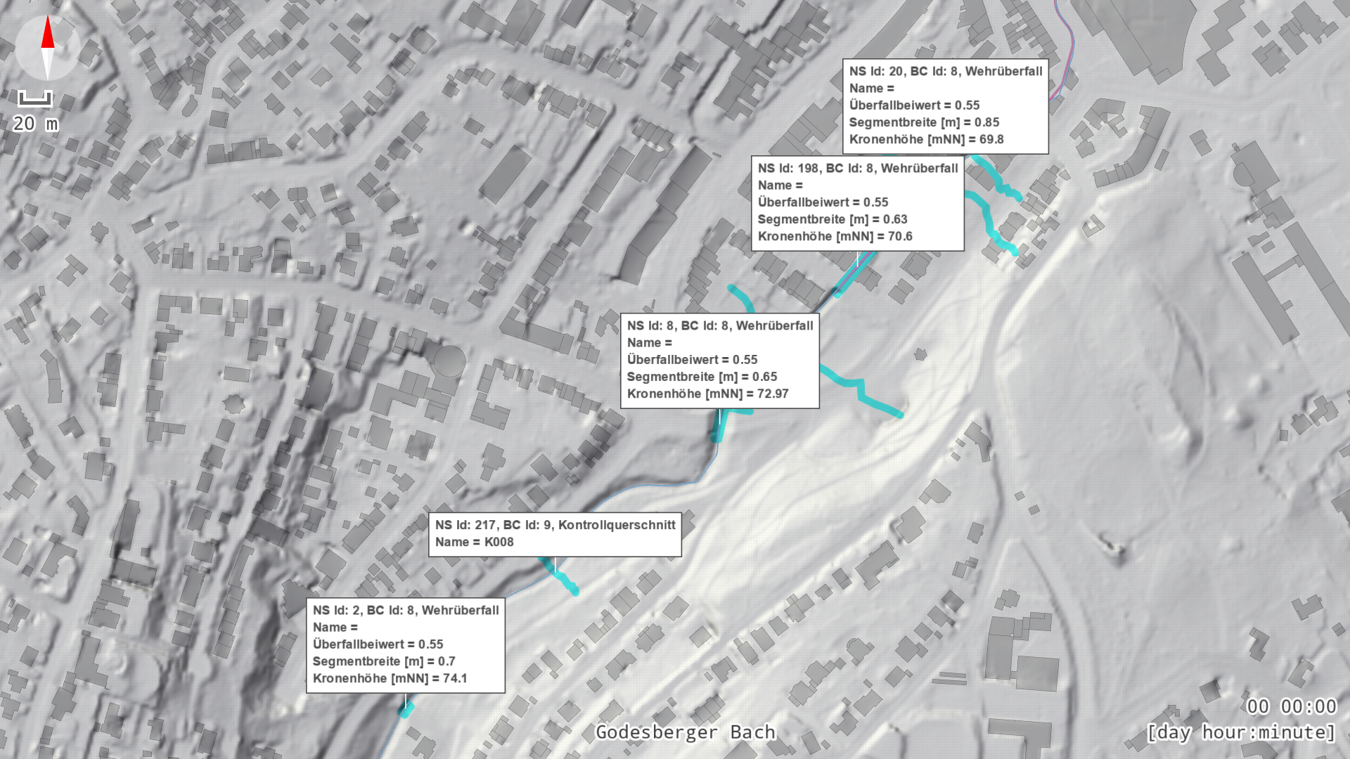
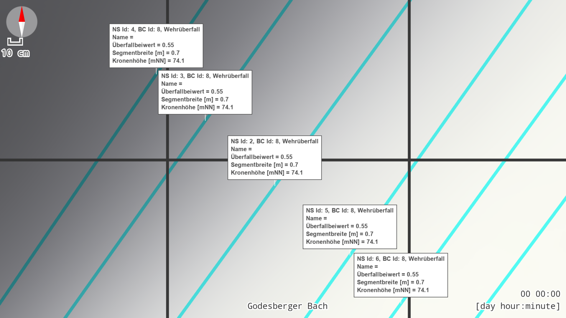
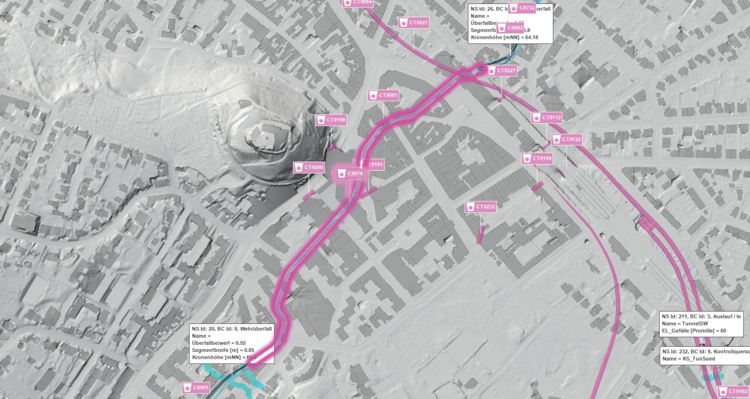
In the Simulation Settings Panel, under Domain Setup – SMS Mesh (.2dm), enable Show NodeString Lines and Show NodeString Labels to visualize all boundary conditions contained in the .2dm file. These appear as cyan line projections on the terrain and as white floating labels above each line, showing the boundary type and associated parameter values.
Because SMS models often contain numerous boundary lines, scenarify applies an intersection-avoidance algorithm to prevent label overlaps.
Use the 2D top-down perspective in the View and zoom in to inspect the labels clearly in specific areas.
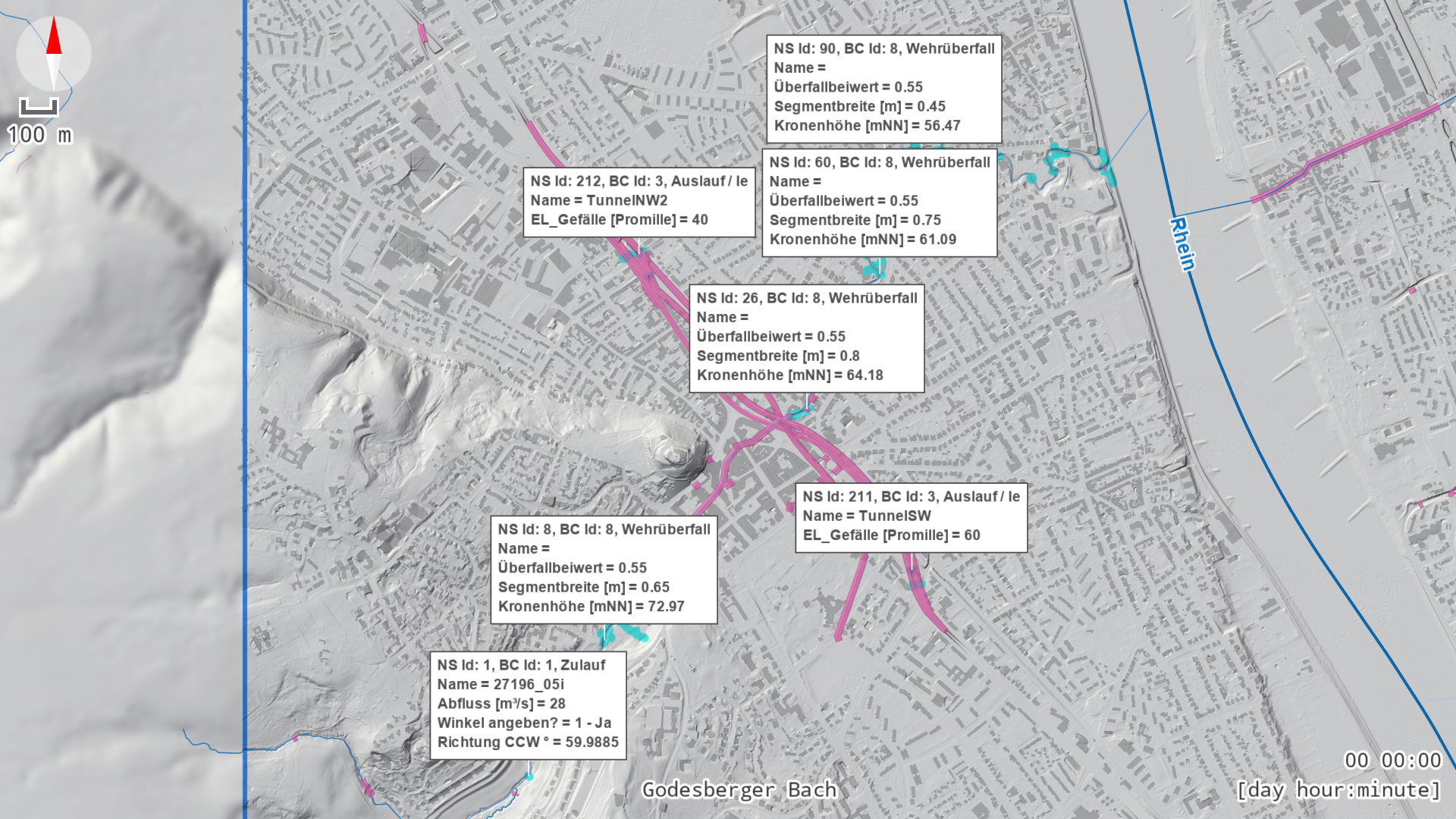
Set Up the Inflow
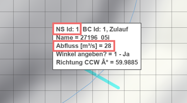
Zoom in to the NodeString with Id 1 ("NS Id: 1") located at the upper end of the river in the View.
Its label contains the name "Zulauf".
Draw an Inflow action along the projected NodeString line, extending it slightly beyond the riverbanks to prevent backflows at peak discharge (see the related recommendations about ensuring proper inflow conditions).
The NodeString label provides hints on the parameters to be used for the inflow.
In this case, the label shows "Abfluss [m³/s] = 28". This value should not be interpreted as a constant discharge.
It represents an identifier for a time series that is stored in the .2dm file.
All time series have been extracted beforehand and are available as a set of CSV files, each named after its identifier.
(See Manually Managed Curves and Time Series for guidance on how to extract these from a .2dm file.)
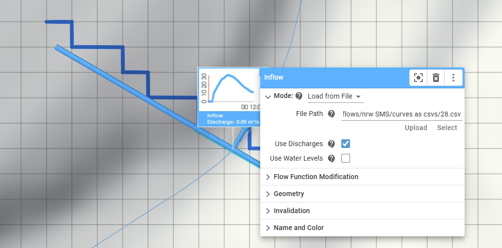
To link the discharge time series:
- Open the Action Settings Panel of the inflow.
- Set the mode to Load from File.
- Select the corresponding CSV file:
Input/taskBasedWorkflows/NRW_SMS/curves_as_csvs/28.csv
The discharge time series is now loaded and displayed in the label plot of the inflow action.
Set Up the Outflow
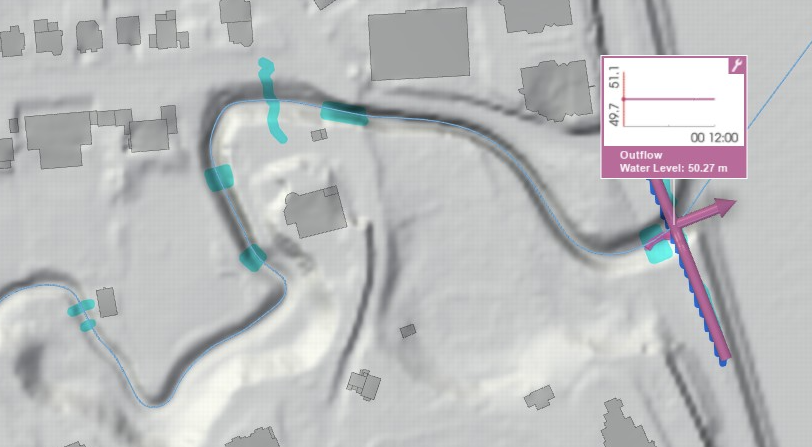
Next, navigate downstream to the point where the river joins the Rhine. Just before the confluence, you will find the NodeString with Id 229 that defines the outflow boundary condition.
Its label reads "H-Randbedingung", indicating that it specifies a water level boundary. The label also contains the entry "WSPL-Zeitreihe = 23", which refers to the water level time series to be used. Note that in this case the water level is constant at 50.27 m, which can also be set up quickly using the outflow mode Enter Water Level.
Draw an Outflow action along the NodeString projection, set its mode to Load from File, and select the corresponding CSV file:
Input/taskBasedWorkflows/NRW_SMS/curves_as_csvs/23.csv
Your model of the Godesberger Bach is now ready for a first simulation.
Click Play to start the simulation and visualize the resulting flood scenario.
4. Apply .2dm Terrain and Roughness
Now, we gradually bring in more details from the .2dm file.
To compare how each modification affects the model and simulation results, we will create a new scenario for every major change.
Create a new scenario based on Godesberger Bach and name it Apply SMS Terrain and Roughness.
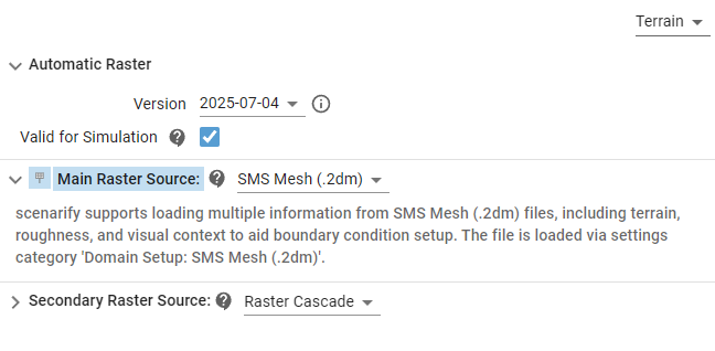
In the Simulation Settings Panel, under Terrain, set Main Raster Source to SMS Mesh (.2dm) and click Run.
The system replaces the automatic terrain from the base model with the geometry from the .2dm mesh wherever valid elevation data is available.
To verify this, toggle between the new scenario and its parent to observe where the terrain has changed.
Set the cell size of the simulation domain to 1 m (for all scenarios that use it) to achieve finer terrain detail.
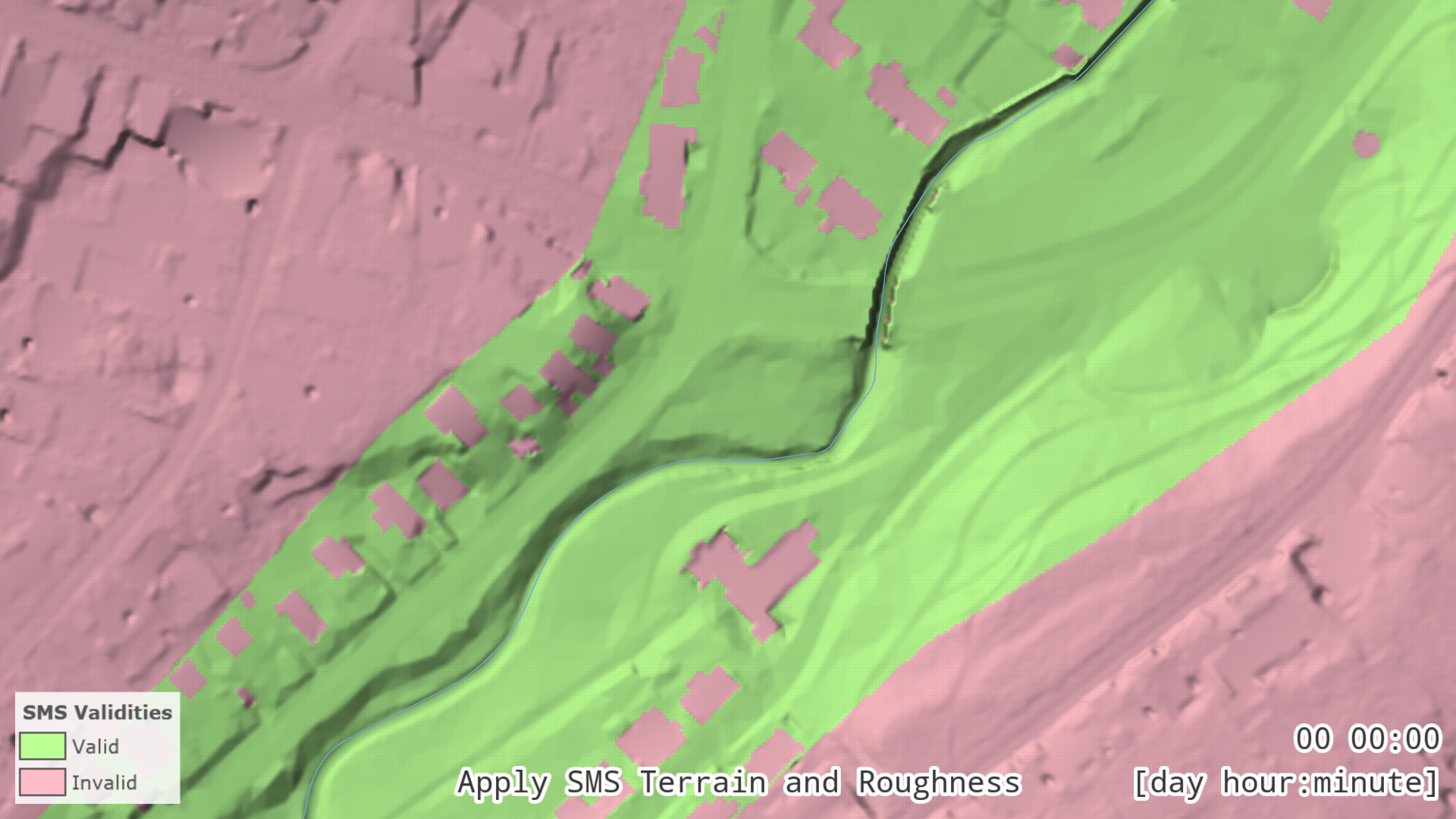
In the Visualization Settings Panel, under Layers: Visualization, in the Terrain row, enable coloring and change the visualization property to Domain Setup: SMS Validities to highlight areas covered by the .2dm mesh.
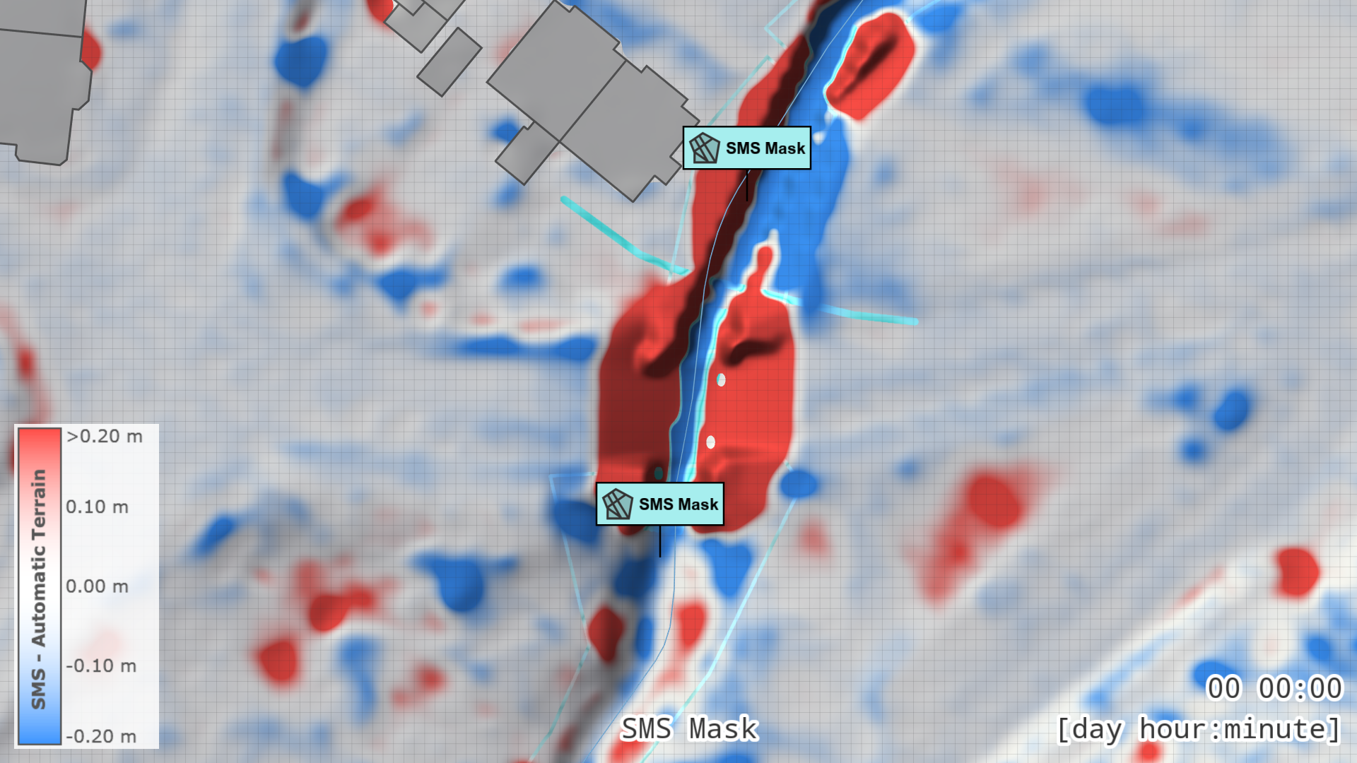
Select the property Domain Setup: SMS vs. Auto Terrain to visualize differences between the imported and the automatically generated terrain.
Red areas indicate where the terrain elevation is higher in the SMS data, while blue areas show higher elevations in the NRW base model terrain.
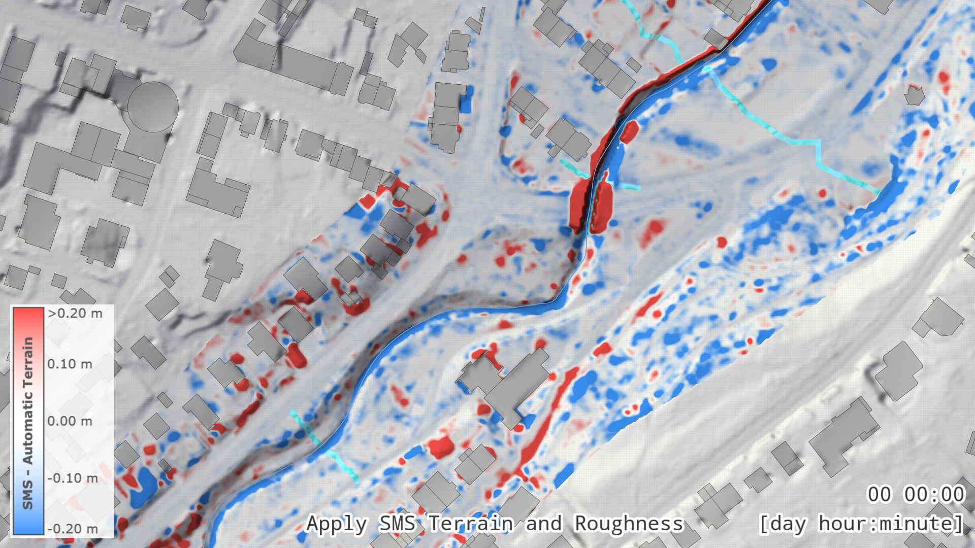
Green areas mark regions where the SMS mesh provides valid data.
Note that projected buildings are turned off in this visualization.
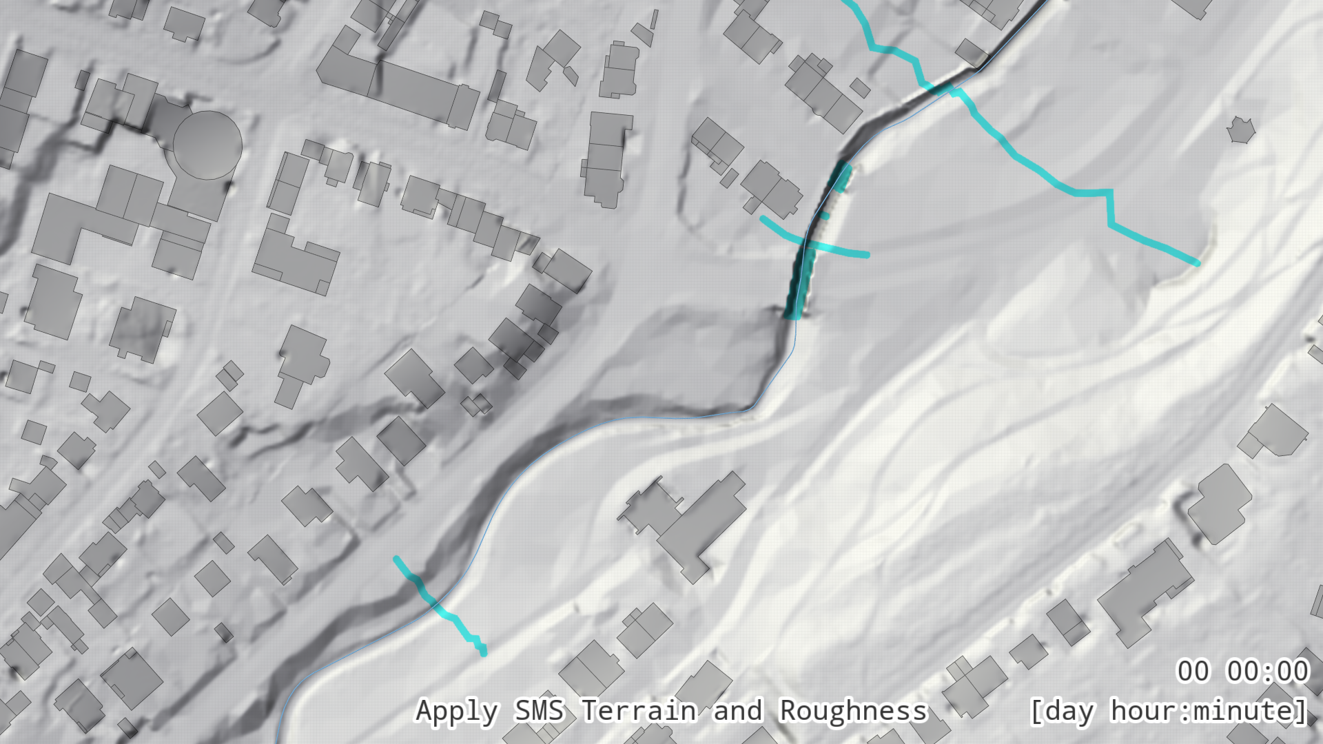
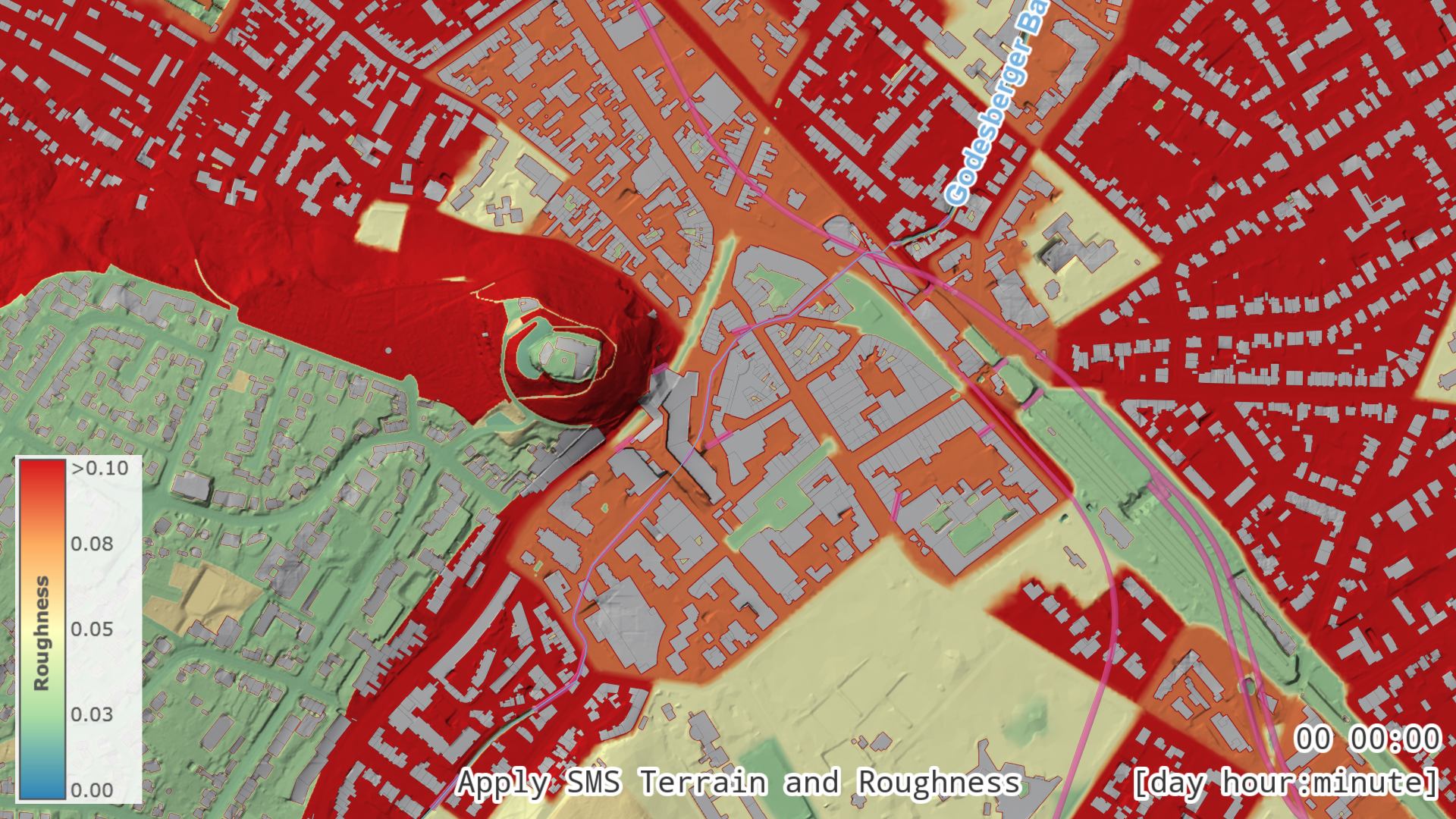
This view shows the terrain without overlay coloring for the scenario "Apply SMS Terrain and Roughness".
It uses the SMS mesh wherever valid values are available.
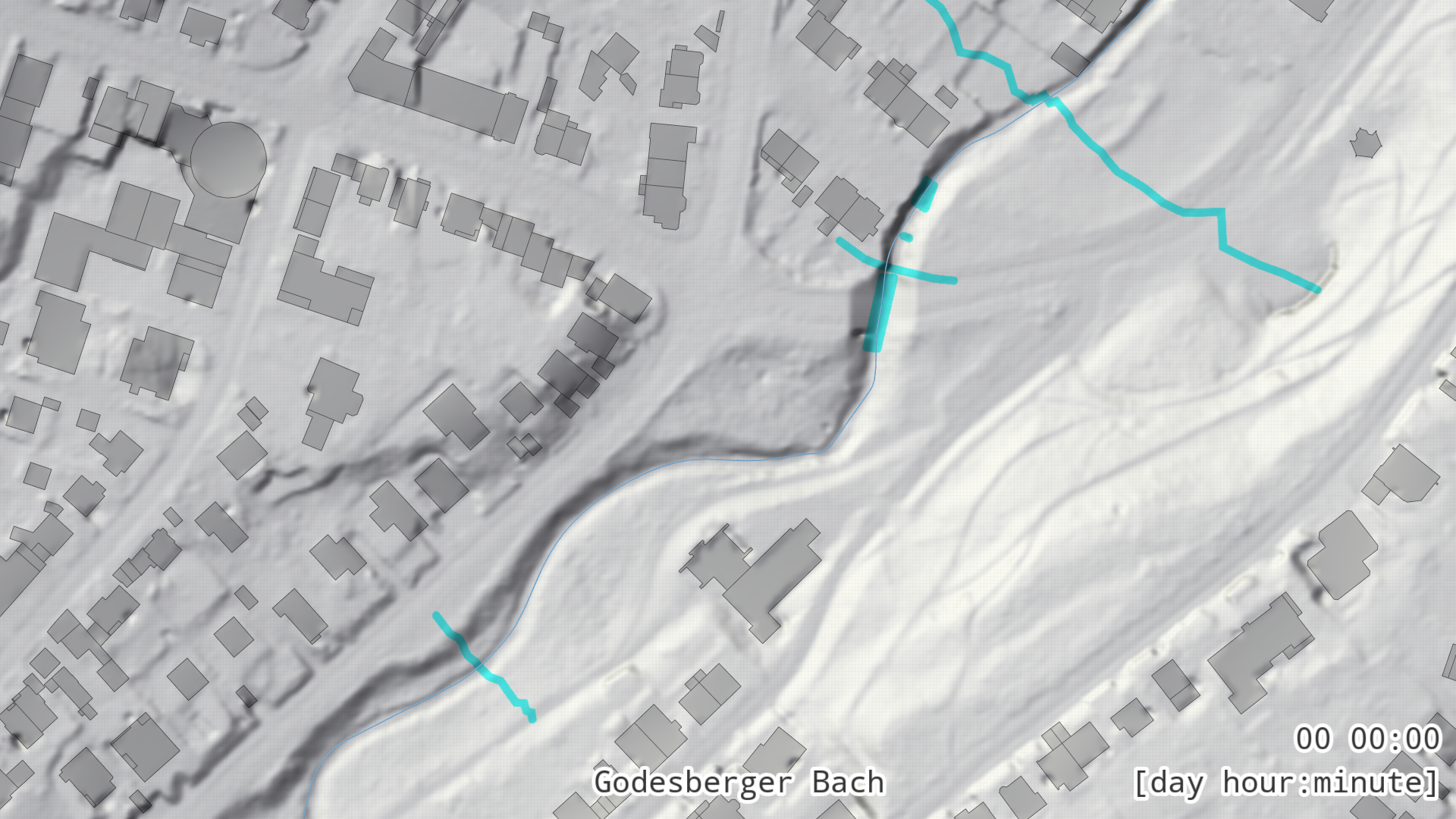
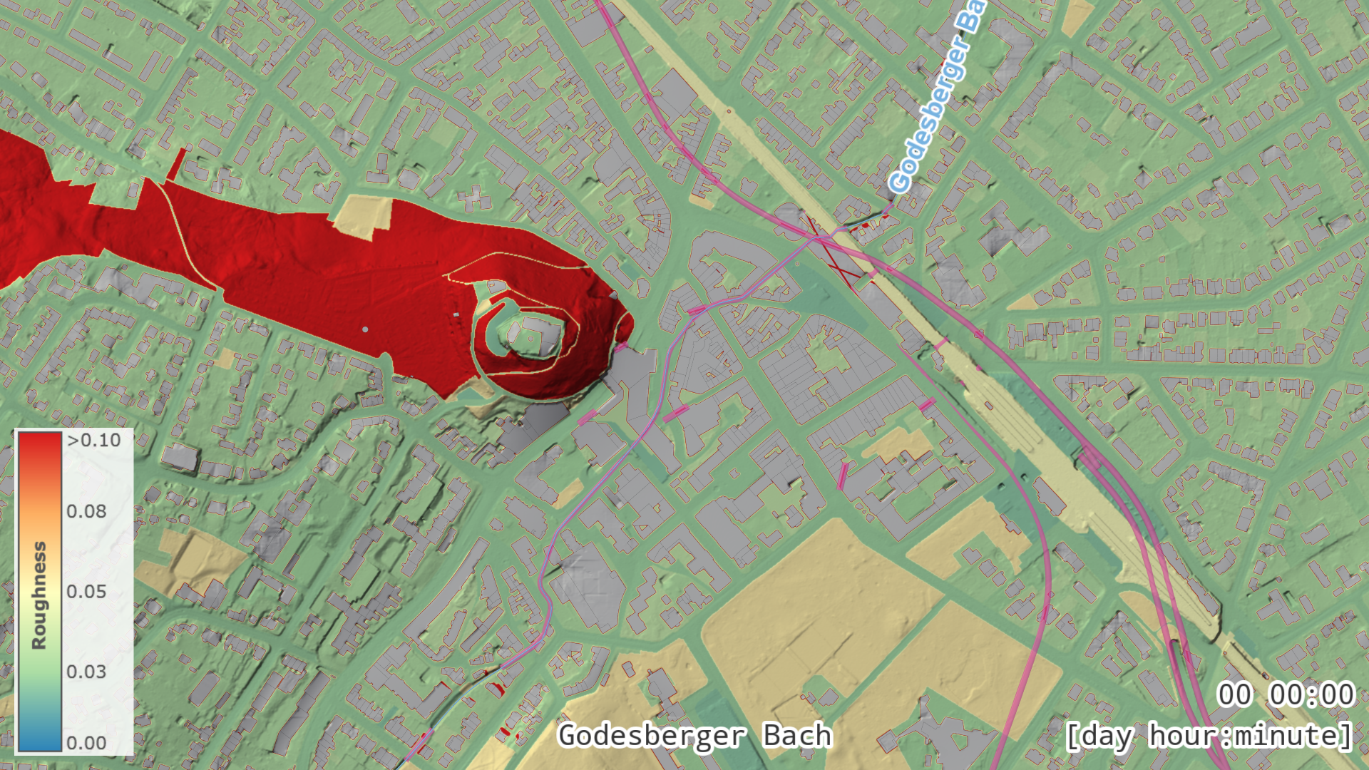
This view shows the terrain without overlay coloring for the scenario "Godesberger Bach".
It displays only the automatic terrain from the base model across the entire domain.
Next, apply the roughness information stored in the .2dm file.
Make sure that the Apply SMS Terrain and Roughness scenario is activated, then open the Simulation Settings Panel under Surface Roughness.
Set Main Roughness From to .2dm Mesh (.2dm) and click Run.
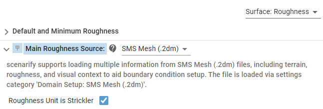
Visualize the roughness distribution using the terrain overlay Surface: Roughness (Manning).
By comparing this scenario with its parent, you will notice that the .2dm roughness values are relatively high.
This likely reflects how the built environment was modeled in SMS.
In scenarify, however, buildings are represented explicitly as wall boundary conditions.
SMS roughness used wherever valid values are available.
The roughness as configured in the base model by default, derived from ALKIS land use data.
All of the following steps further increase the level of detail in the model.
They are considered optional, and it is up to the modeller and the specific use case objectives to decide which steps are necessary.
5. Masking (Optional)
One of the most important geometric features we want to extract from the .2dm file is the riverbed, which ideally represents measured terrain data.
However, outside the river channel—in the surrounding floodplain—the mesh is often much coarser due to external simulation performance reasons.
In these areas, the scenarify base model terrain generally provides a higher level of detail.
In addition, buildings may be integrated directly into the .2dm geometry, with roughness values used to represent built-up areas. In scenarify, by contrast, buildings are modeled explicitly as wall boundary conditions, which supports more accurate flood impact analysis.
For these reasons, we do not want to apply the .2dm geometry and roughness everywhere they are valid.
Instead, we limit their influence to the riverbed region, while preserving the higher-resolution base terrain elsewhere.
To support this workflow, scenarify provides several ways to mask the .2dm geometry and roughness:
- Masks loaded from polygonal Shape files
- Masks derived from land use or riverbank data already setup in the model
- Manually drawn mask actions
- Or any combination of these methods
Import SMS Mask Actions
All masking options are managed through the SMS Mask action (see its action description for details).
Ideally, you may already have mask polygons available as shapefiles from previous projects.
In this example, we will create a mask based on land use data that is already included in the NRW base model (derived from the federal ALKIS land use dataset).
Create a new scenario based on Apply SMS Terrain and Roughness and name it SMS Mask.
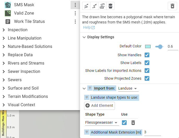
In the Action Tool Panel of the SMS Mask action, set Import from: to Landuse.
In the table below, add the following land use type to include: Fliessgewaesser.
We want the .2dm mesh to extend slightly beyond the riverbed, so set Additional Mask Extension to 3 m.
This applies a 3-meter buffer around each polygon.
Note that this operation is geometric and may take longer to compute for large or complex polygons.
In the ALKIS dataset, the riverbeds are already divided into smaller segments, so the algorithm runs efficiently.
Click Run to apply the mask.
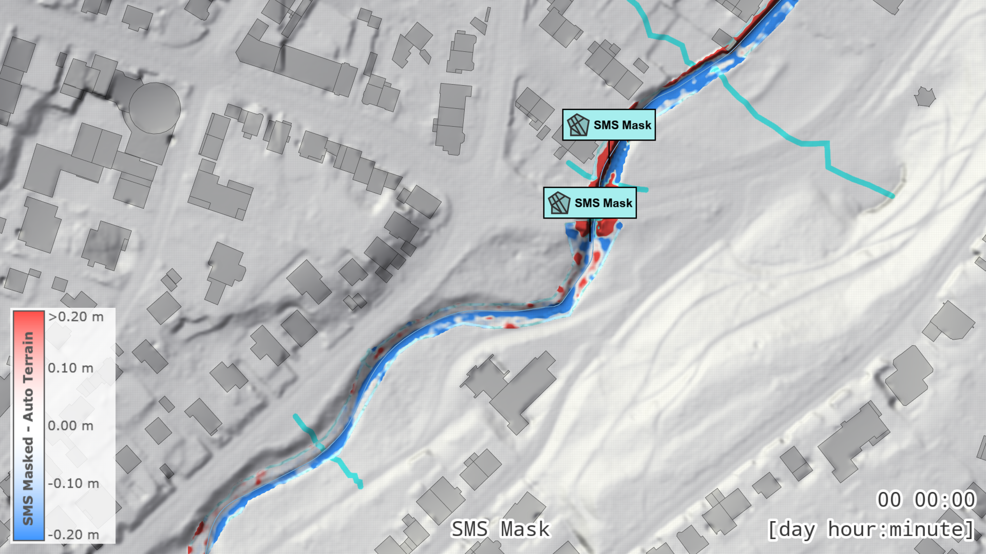
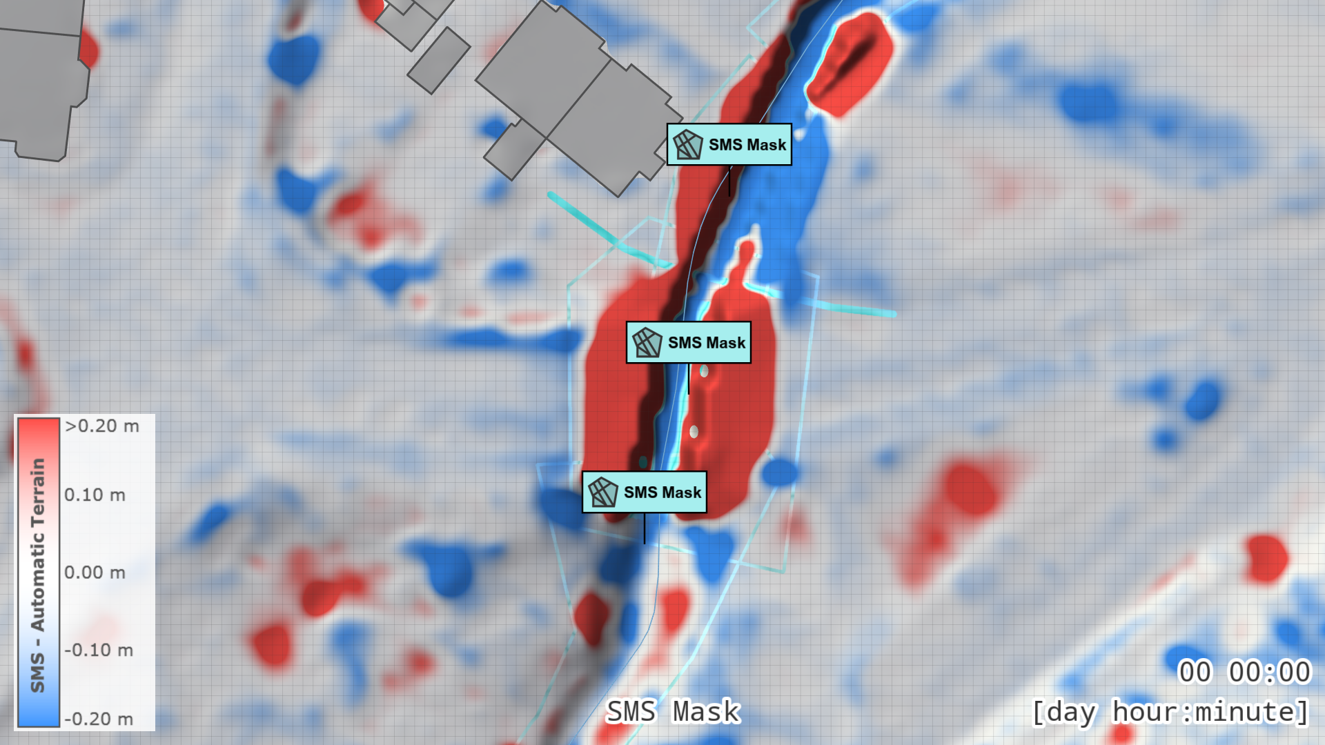
The .2dm geometry is now applied only within the masked area.
Use the terrain visualization property SMS Masked vs. Auto Terrain (Difference) to compare the automatic terrain and the .2dm terrain within the masked regions.
Fine-Tuning the Mask
Fine-tuning may involve editing, removing, or adding masks as needed. Use the terrain visualization property SMS vs. Auto Terrain (Difference) as visual context for this work.
-
Remove unnecessary masks and edit masks
Edit or delete masks using the additional action creation modes of the SMS Mask action.
In particular:- Remove masking over side arms of the Godesberger Bach that are not explicitly covered by the .2dm model.
- Reduce the mask extension where it includes buildings located directly along the river.
-
Add missing masks
In some areas near bridges, the automatically loaded masks may not fully cover the modeled geometry. For example, at bridge locations, the approach ramps on both sides of the river are represented in the .2dm geometry. Draw additional masks to include these regions.
Once the masking setup is complete, you can hide all SMS Mask labels in the Action Tool Panel of the SMS Mask action to reduce visual clutter in the View.
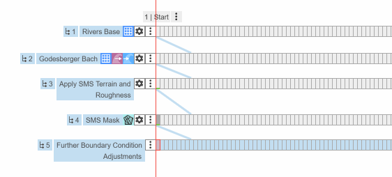
For the remaining optional steps, create a new scenario based on SMS Mask and name it Further Boundary Condition Adjustments. Your scenario hierarchy should now look like in the image below. Feel free to create additional scenarios for each step if you want to compare in more detail how each modification affects the simulation results.
6. Culverts Editing (Optional)
The NRW base model includes a statewide set of culverts derived from federal ATKIS data using AI-based algorithms. Culverts located in riverbeds have their cross-sections derived from the corresponding riverbed profiles. You may want to fine-tune these culverts based on parameters and geometry information extracted from the imported .2dm file.
Edit or remove culverts using the additional action creation modes of the Culvert action.
Inspect the NodeString labels in the .2dm view to gather hints on the appropriate parameter settings.
In this tutorial, we examine several specific cases.
To help you locate them in your model, we refer to both the NodeString ID (shown in the top-left corner of each NodeString label) and the internal scenarify name of the corresponding Culvert action.
To view the latter, switch to Edit Mode.
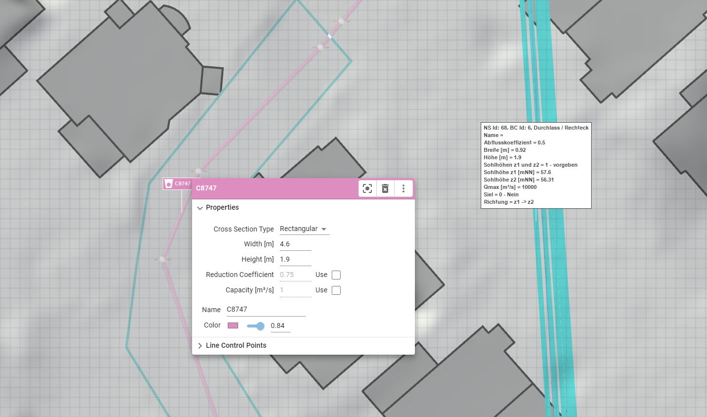
Case 1: NS Id 86 — Culvert C8747
The scenarify culvert C8747 already follows the actual underground pipe alignment well, so no changes are needed to its position.
In the SMS model, this culvert is represented by a set of five NodeString boundaries. Since SMS can only connect two mesh nodes per boundary, these were used to approximate the full extent of the culvert.
To fine-tune the cross-section of the corresponding rectangular culvert in scenarify, refer to the NodeString parameters:
the height is 1.9 m and the width is 0.92 m.
Multiply the width by 5 (to reflect the five NodeStrings) to obtain a total width of 4.6 m.
Edit the culvert, set its cross-section type to Rectangular, and update the width and height accordingly.
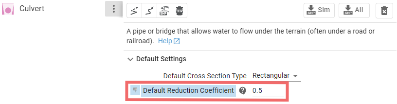
Default Parameter Adjustment for All Culverts
All NodeString labels representing culverts indicate the use of a discharge reduction coefficient (Abflusskoeffizient) of 0.5, whereas scenarify uses 0.75 by default.
Open the Action Tool Panel and adjust this value for all culverts at once to 0.5 to match the SMS setup.
Case 2: NS Id 215 — Culvert C8876
This culvert represents a particularly long underground section of the Godesberger Bach.
In the SMS model, it is modeled using an outflow boundary controlled by a rating curve, which connects to an inflow boundary at the other end of the structure.
This approach requires knowledge of the rating curve or at least the energy slope, which is typically only available at gauged stations.
In scenarify, this situation is modeled directly as a Culvert action, where the pipe geometry affects the discharge capacity. Edit culvert C8876 and reduce its width to 3.6 m.
Case 3: Long Culverts Representing Tunnels (e.g., CT2907)
For long culverts that represent tunnel sections, you can either keep or fine-tune the existing culvert actions.
To replicate the SMS model more closely, you may instead remove these culverts and create Invalid Zone actions at the tunnel entrances.
Alternatively, if the energy slope is known, you can replace them with Outflow actions exactly like in the SMS configuration.
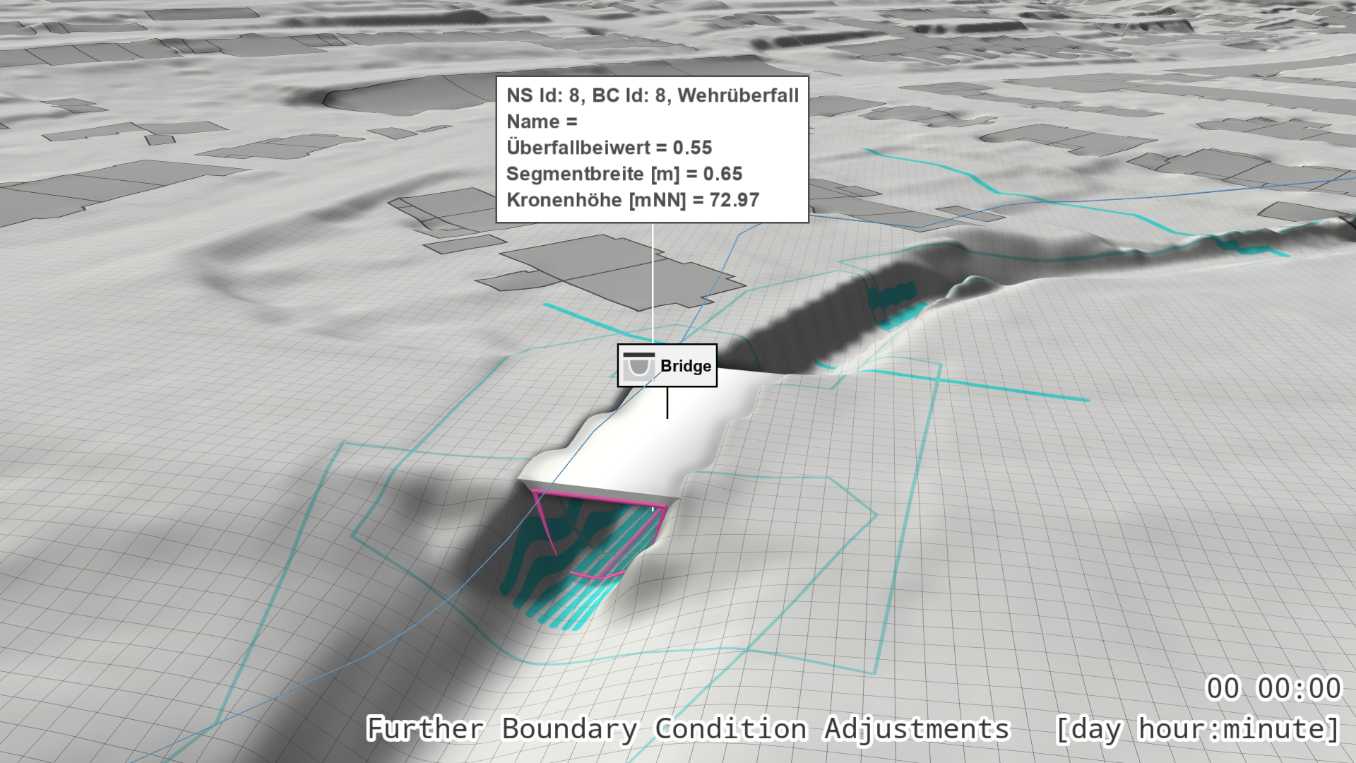
7. Bridges (Optional)
In the SMS model of the Godesberger Bach, several bridges are represented as weirs (for example, NS Id 8).
In the NRW base model, bridges are typically either cut out or modeled as Culverts, which already ensures flow continuity in most rivers.
In contrast, the SMS model uses Weirs to represent bridge structures.
To better capture bridge behavior in scenarify, allowing for flow beneath the deck and overtopping flow above, as well as flow obstruction by the deck, it is recommended to use the Bridge action.
Let’s apply this for NS Id 8:
Ensure that an SMS Mask is active in this area so that the side parts of the bridge geometry from the .2dm mesh is available.
Draw a Bridge action as a polygon enclosing the bridge’s side sections.
The bridge deck top elevation is automatically derived from the underlying terrain.
Only the bridge deck thickness needs to be set manually in the Action Settings Panel.
Repeat this procedure for other bridges along the Godesberger Bach as needed.
If a bridge location already contains a culvert from the base model, remove it before adding the Bridge action.
8. Protection Lines (Optional)
In SMS, thin wall structures are typically embedded directly into the mesh.
In scenarify, these are represented as wall boundary lines, which preserve overtopping elevations regardless of the simulation cell size.
This vector-based representation also provides greater flexibility for modeling scenarios such as protection wall breaches, and makes future terrain updates easier to manage.
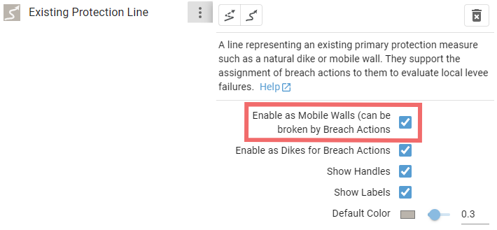
Existing protection lines can be imported as 3D line shapefiles in the Simulation Settings Panel under Barriers: Existing Protection Lines. Within this panel, you can enable Protection Lines as Walls to represent them as mobile walls (By default, these lines are used only to delineate dike structures in the terrain).
Alternatively, you can create protection lines manually using the Existing Protection Line action.
Other barrier types, such as Concrete Walls (abs), can also be used. These support both manual drawing and loading from shapefiles. If you draw Concrete Walls (abs) manually on top of the SMS mesh, make sure to set the Default Height to 0 in the Action Tool Panel of Concrete Walls (abs).
In this tutorial, we assume that no vector data is available, so we will draw the protection line manually.
We use the mesh visualization as a guide, drawing the line directly over the .2dm mesh to capture both the correct location and elevation.
In the Simulation Settings Panel, under Domain Setup: SMS Mesh (.2dm), enable Show Mesh.
If you want to avoid visual artifacts caused by the terrain and mesh intersecting, you can temporarily hide the terrain layer in the Visualization Settings Panel under Layers: Visualization.
When drawing the protection line as a polyline, remember that any abrupt height changes require two control points before and after the step to correctly interpolate the 3D line.
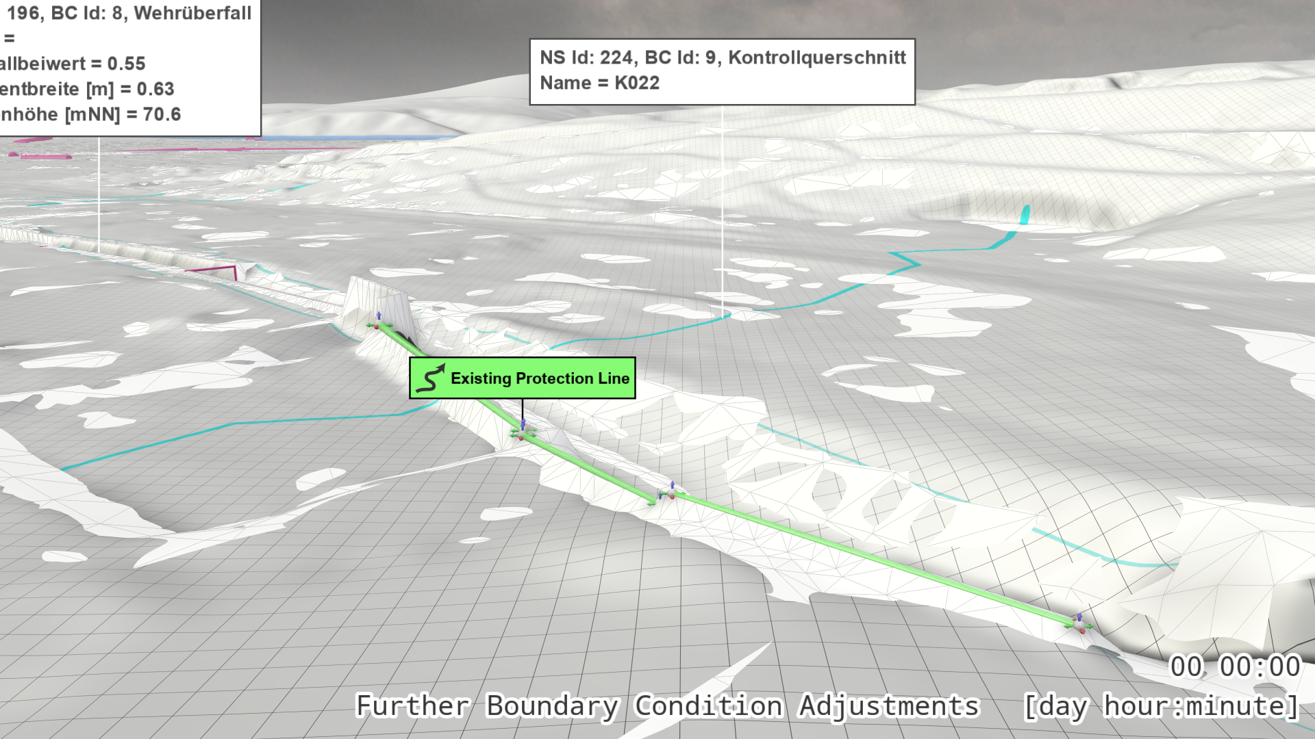
In this example, draw an Existing Protection Line along the thin wall structure that runs parallel to the Godesberger Bach and intersects the NodeString with ID 224 (a control profile or "Kontrollquerschnitt").
In the Action Tool Panel of the Existing Protection Line action, enable Mobile Walls (can be broken by Breach Actions).
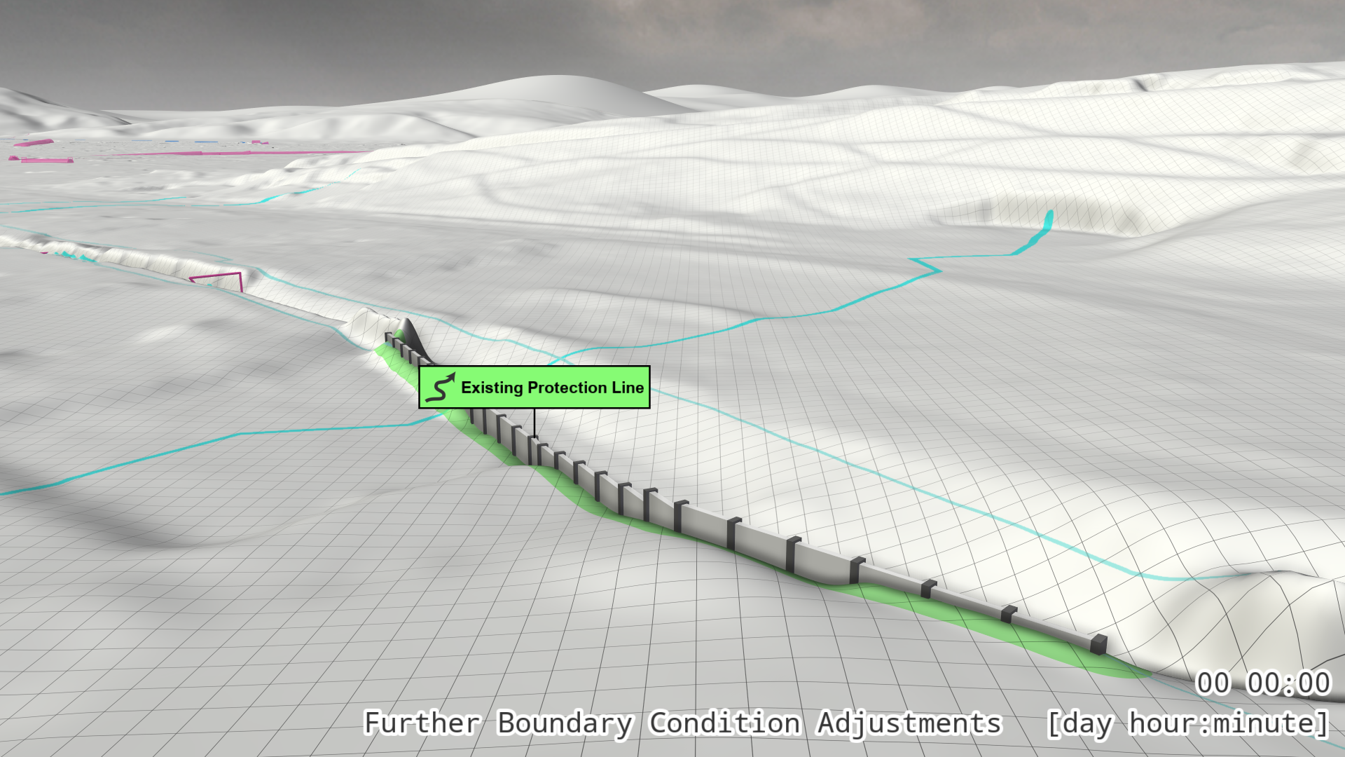
In the View, mobile wall segments will appear along the line, extending up to the elevation defined by the protection line.
An Existing Protection Line drawn on the SMS mesh, colored green for visibility.
The Existing Protection Line action represented as mobile walls.
9. Initial State (Optional)
scenarify provides several methods for defining an initial state within the river bed.
If the automatic terrain is derived from a laser scan that includes the water surface (as in the NRW base model at the time of writing), while the .2dm file contains a cut-out riverbed, you can easily generate an initial state for your simulation by exporting the automatic terrain inside the SMS masks.
In the Simulation Settings Panel, under Layers: Visualization, select the terrain visualization property Domain Setup: Auto Terrain in SMS Mask and export it.
The resulting raster can then be re-imported in the Simulation Settings Panel, category Surface: Initial State.
Working with Large or Multiple .2dm Files
If you are working with a .2dm file that covers a large domain, it is recommended to use temporary, smaller simulation domains with a resolution suitable for the interactive work described above.
This will improve responsiveness during editing and visualization.
See also our guidelines on
If you need to integrate multiple .2dm files into a single scenarify model, for example, if a river is split into several separate SMS projects, you can follow this workflow.
1. Applying Terrain and Roughness
When integrating several .2dm files, you first need to extract the terrain within the riverbeds from each file.
There are three options for doing this:
a. Export masked terrain, roughness, and initial states from scenarify
- For each imported .2dm file, apply the masks as described earlier.
- Export the masked terrain, roughness, and initial state using the visualization properties Domain Setup: SMS Masked Terrain, Domain Setup: SMS Masked Roughness, Domain Setup: Auto Terrain in SMS Mask.
- Repeat this process for each file and collect the exported GeoTIFF raster files in separate folders for terrain, roughness, and initial state.
- Later, re-import them as Raster Tiles for the main terrain or roughness source.
b. Use QGIS to process .2dm files externally
- The free GIS software QGIS can read .2dm files and apply masks if polygon layers are available.
- You can export masked .2dm layers from QGIS as GeoTIFF raster files, which can then be imported into scenarify as Raster Tiles.
c. Request batch conversion
- If you have many .2dm files along with mask polygons with sufficient quality, you can contact us at scenarify@vrvis.at.
We can convert them into raster tiles for you using an automated batch process.
2. Integrating Boundary Conditions
When combining multiple .2dm files, always work within the same scenarify project, processing one file after another.
Create one or more base scenarios to collect all created actions on them (for example, all culverts or bridges).
On top of these base scenarios, create your actual simulation scenarios with dedicated simulation domains.
See also our recommendations on using the domain as a scenario parameter.
If you plan to create river flood maps for a large region, refer to our guidelines on river flood modeling for large regions.
Comparison with External Simulation Results
If you need to compare scenarify simulation results with those from another hydraulic model, there are several aspects to consider.
The scenarify team has carried out such comparisons multiple times and can share a few best practices. To achieve sufficiently equivalent results, keep the following points in mind:
- The external model must also solve the 2D shallow water equations, as scenarify does.
- Use the same terrain and roughness configuration.
If you want directly comparable results, avoid masking and use the thinned-out mesh even outside the riverbeds. - Choose a sufficiently small cell size for the simulation domain to ensure similar spatial resolution.
- Identify the global simulation parameters used in the external model and reproduce them in scenarify.
Important parameters include:- Solver accuracy: first order corresponds to interactive accuracy in scenarify, while second order corresponds to high accuracy.
- The use and configuration of water-depth-dependent roughness.
- Apply all setup steps with respect to boundary conditions carefully, as they can influence comparability.
- Be aware that different simulation tools may treat boundary conditions differently in their numerical implementation.
You might need to adjust scenarify action parameters, such as reduction coefficients, to achieve comparable behavior.
Visual Comparison
To support calibration in scenarify, you can overlay externally simulated maximum water depths as visual context on the terrain.
Import the external results as a custom raster in the Visualization Settings Panel under Setup Visual Context: Custom Raster. In the Layers: Visualization category, set the terrain visualization property to Visual Context: Custom Raster to display the imported data.
For a direct comparison with the maximum water depths simulated by scenarify up to the active time step, select Visual Context: Max. Depths – Custom Raster to show the difference.
Supported SMS Tags
scenarify reads and interprets the following tags from .2dm mesh files:
Automatically Parsed Tags
| Tag | Description / Purpose |
|---|---|
| E3T, E4Q | Define mesh elements (triangles or quadrilaterals) by referencing their node IDs. These form the main 2D computational domain. |
| ND | Defines a node in the mesh with its coordinates (x, y, z). |
| NS | Defines a NodeString, a connected sequence of nodes used to mark inflows, outflows, monitoring cross-sections, or other boundary conditions. |
| BC, BD | Define boundary conditions — they link physical meaning (e.g., inflow, outflow, culvert) and parameters to a NodeString. |
| BC_DEF | Describe which parameters belong to each boundary condition type, including their names and units (e.g. "Discharge [m³/s]"). |
| BC_VAL, BCS | Assign specific parameter values to a boundary condition. For example, a fixed discharge or a reference to a time series curve. |
| MAT | Defines material zones — each element of the mesh belongs to one material. Materials control hydraulic roughness. |
| MAT_DEF | Defines the type of roughness parameter used (e.g. Strickler or Manning). |
| MAT_VAL | Assigns actual material parameter values (e.g. Strickler Kst = 30 m¹ᐟ³/s or Manning n = 0.033). |
Manually Managed Curves and Time Series
scenarify does not automatically link or parse time-dependent data.
If your .2dm file contains discharge or water level time series, or rating curves (w–Q curves), you can extract the required data manually by opening the file in a text editor and saving the relevant sections as .csv files for use in scenarify. Ensure that your .csv files follow the format specifications.
| Tag | Description / Purpose |
|---|---|
| XYS | Defines a time series (e.g. discharge or water level) as pairs of values (time [s]; value), or rating curves. Each curve can be referenced by ID from a boundary condition (BC_VAL S). |
| TIME | Marks time-related information or blocks in older .2dm formats. Treated the same way as curves and must be exported manually. |
Tip: You can use an AI assistent such as ChatGPT to extract and convert curves directly from your
.2dmfile. Simply upload your file and ask something like: "Generate one CSV file per time series (XYS) in this.2dm, named after the curve ID (e.g.2.csv), with the headerTime<double>[s];Discharge<float>[m³/s]." The AI assistant will provide you with a downloadable.zipfile containing all the curve data. It may be necessary to adjust the header in the resulting CSV file, e.g., if water levels are stored instead of discharge values.