Comparison and Calibration with Measurements
When developing models, whether for hydrological, hydraulic, or other environmental systems, it is crucial to validate and fine-tune them using real-world data. Comparison with measurements ensures the model reflects observed conditions, while calibration adjusts model parameters to improve its performance by modifying specific parameter (e.g. roughness coefficients) to align simulated outputs with measured data, such as water levels. This process enhances accuracy, reliability, and the predictive capabilities of your simulations.
Roughness Calibration
Roughness calibration is needed to adjust the friction term in hydraulic models, allowing for more accurate representation of water flow. For this hands-on practice, we assume you already have a working river flood model set up. Follow these steps to calibrate the roughness coefficient for a river flood scenario, assuming measured data from multiple gauges is available.
1. Create Spatial Inspections
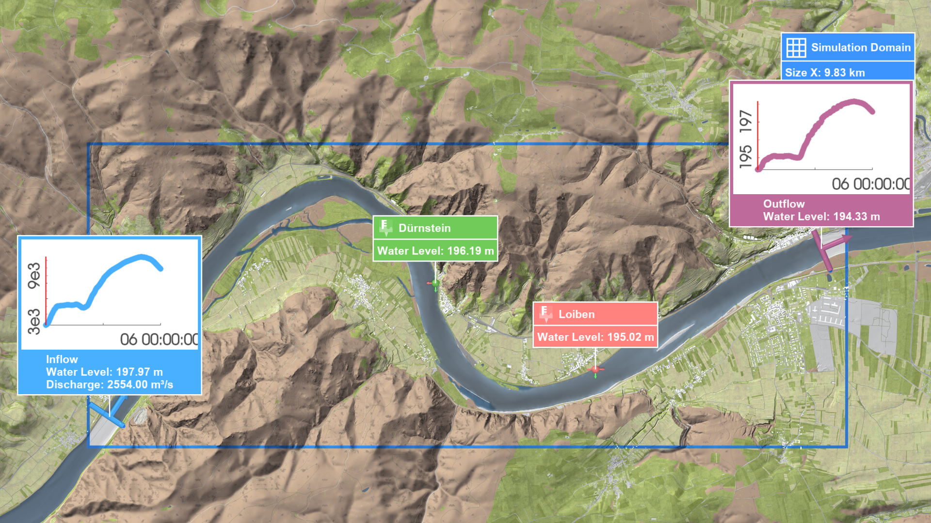
Draw Spatial Inspections at the gauge locations. These inspections will extract simulated water levels, enabling comparison with the measured data.
Hint: To display river cross sections at gauge locations from a shape file, use Custom Lines in the Visualization Settings Panel under Setup: Visual Context. This can be useful for drawing inflow, outflow, and spatial inspections.
2. Assign Measured Water Levels
Next, in the Action Settings Panel for each Spatial Inspection, select the CSV file containing the measured water levels and assign it a descriptive name:
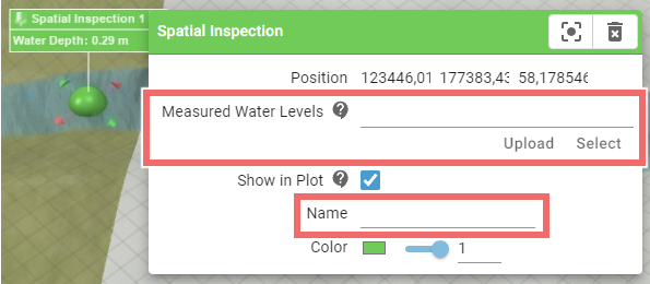
The measured water level time series need to be provided as CSV Files with the following columns: Time and Water Level. Here is an example:
Time<time>[];Water Level<float>[m]
10.05.2013 23:00;103.94
10.05.2013 23:05;103.96
10.05.2013 23:10;104.97
...
3. Run Multiple Scenarios with Different Roughness Coefficients
To calibrate roughness, multiple scenarios with varying riverbed roughness values to assess how these roughness changes affect simulated water levels. These scenarios will help you determine which roughness coefficient best matches the measured data. For accurate river flood simulations, it is recommended to use High Accuracy for River Floods in the Surface: Simulation Model settings.
A best practice is to set up a common parent scenario, such as Comparison Base. Then create multiple scenarios with this scenario as parent and adjust parameters like the roughness coefficient for the riverbed ("Fliessende Gewässer") in the roughness from landuse mapping:
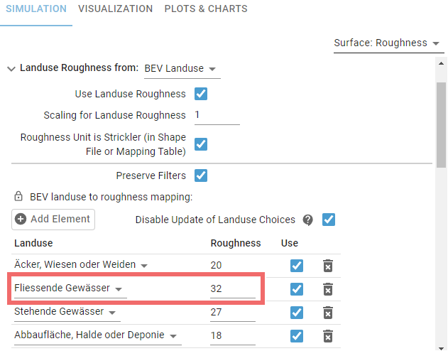
By default, changes to roughness are applied to the active scenario. After creating several scenarios with different roughness values, your scenario hierarchy should look like this:
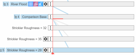
You can either run each scenario individually or use the Batch Processing interface to run multiple scenarios simultaneously. This will generate water level time series data, which can be compared against the measured water levels to identify the optimal roughness coefficient.
4. Compare Simulated and Measured Water Levels
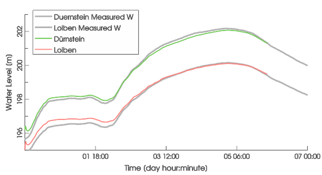
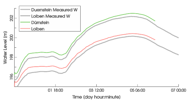
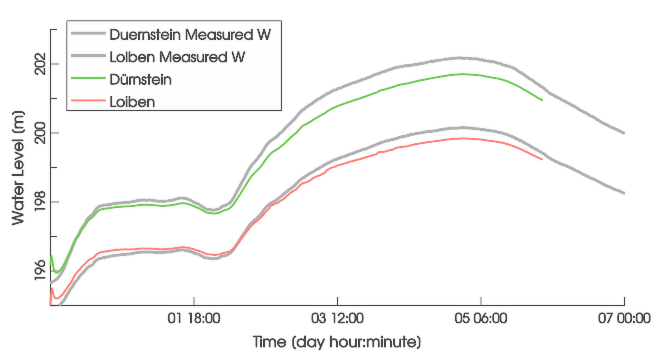
To visually evaluate how well each scenario matches real-world water level measurements, use the Inspection: Water Level plot in the Plots & Charts panel. This plot allows you to compare simulated water levels against the measured data:
Hint:
To calculate a metric like the RMSE (Root Mean Square Error) for each scenario in your preferred external tool, export the simulated water levels for all Spatial Inspections simultaneously using the CSV Export button in the Action Tool Panel:
The exported CSV files contain time series data for each spatial selection, while the SHP file includes the locations of all spatial selections as 3D positions (PointZ).
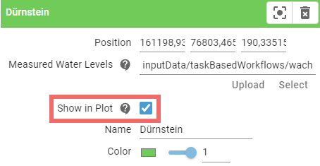
To display only selected Spatial Inspections in the plots, enable Show in Plot for those actions:
5. Pick the Best Fit
After comparing the results, select the scenario that shows the best match between simulated and measured water levels. The scenario with the closest alignment will have the optimal roughness coefficient, ensuring your model accurately represents the river's hydraulic conditions. In the example above, the measured flood peak is best captured with a Strickler roughness coefficient of 32 m^(1/3)/s.
This completes the task-based workflow for roughness calibration in river flood modeling. Special thanks to via donau - Österreichische Wasserstraßen-Gesellschaft mbH for providing the gauge data used in this example.
Runoff Calibration
Similar to roughness calibration, infiltration parameters like saturated hydraulic conductivity can be adjusted to improve model accuracy. This is done by using Profile Inspections to compare simulated and measured discharges at catchment outlets. The Inspection: Profile Discharge plot allows you to visually assess how well the simulated runoff matches the observed data, enabling effective calibration of infiltration parameters.
